
In this tutorial, we will know what is Excel SUMPRODUCT along with the syntax, arguments, return value and why use this function. Thus, we will cover ways how to use SUMPRODUCT from basic to multiple criteria wherein we will know the difference between the Sum and SUMPRODUCT.
To begin with, let’s define what is SUMPRODUCT…
What is the SUMPRODUCT function in Excel?
SUMPRODUCT function in Excel multiplies the two numbers, arrays or ranges and sums up the products. Thus this function is used to calculate the weighted average.
Additionally, this function is very handy the same with is versatile which can be used to count and sum such as COUNTIFS and SUMIFS this made the function more flexible.
Aside from being flexible, this function can handle arrays in various ways wherein functional to compare data with different ranges.
Hence, it can calculate multiple criteria. So here is the syntax with its arguments and return value…
Syntax
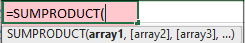
Arguments
- array1 – required argument which is the array or range to multiply.
- array2, array3 – an optional argument which is the second or third arrays to multiply and ad.
Return Value
The return value is the multiplied and summed arrays or ranges.
Why Use SUMPRODUCT?
Using SUMPRODUCT helps you calculate your weighted average and many financial analysts use this function to determine the difference in comparing two data.
At first use, this function may look boring, and complicated. However, if you know the work of this function, as well as master this skill you will amazingly see how versatile this function is. Hence this function easily handles the arrays and range of cell processes.
How To Use SUMPRODUCT in Excel
Time needed: 3 minutes
This time we will know how to use SUMPRODUCT in Excel on its basic usage before proceeding to multiple criteria which is a bit complex.
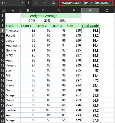
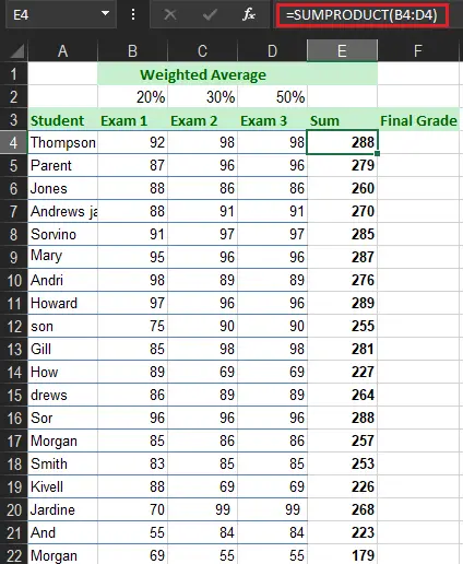
- In this case, we get the Sumproduct of final grades of the student.
So the SUMPRODUCT dis is multiplied the 20% to the first exam, then 30 % to the second exam and 50% to the third exam, sum up the product of each array.
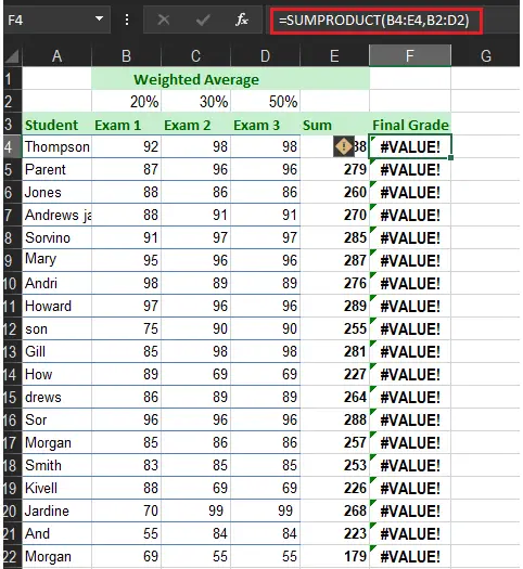
- The range must be proportioned. If not it will return the result #VALUE! error.
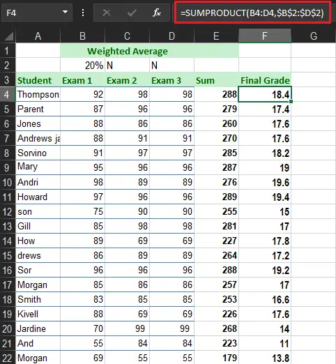
- The SUMPRODUCT determines the text string as zeros.
- If it is a single range the result of SUMPRODUCT is the same as the SUM function.
Double — negative Sign
The double negative (–) is used to force TRUE and FALSE values in numeric equivalents which are 1 and 0. If we have 1 and 0 in our data we can execute many operations on the arrays together with Boolean logic.
Hence, the table below displays the array1 and array2 wherein the double negative the true or false values into 1 and 0.
| array1 | array2 | Product | ||
| 0 | * | 50 | = | 0 |
| 0 | * | 75 | = | 0 |
| 1 | * | 150 | = | 150 |
| 0 | * | 85 | = | 0 |
| 1 | * | 250 | = | 250 |
| Sum | 400 |
Excel SUMPRODUCT Multiple Criteria
The SUMPRODUCT with multiple criteria is used to compare multiple arrays with various criteria. The thing to remember is the same format of the SUMPRODUCT with multiple criteria. Although it will consist of two or more ranges.
Additionally, you can use this function instead of using COUNTIF, SUMIF and etc. Thus, it is used to create a complex formula that sums up the arrays’ rows and columns. Along with it works with logical functions like AND, OR, & both.
Example 1:
So here we are going to use this function corresponding to the multiple criteria. This time assuming we have the data which contains the business sales.
The following are the steps to do multiple criteria:
- Below are the sample data we going to use in SUMPRODUCT function.
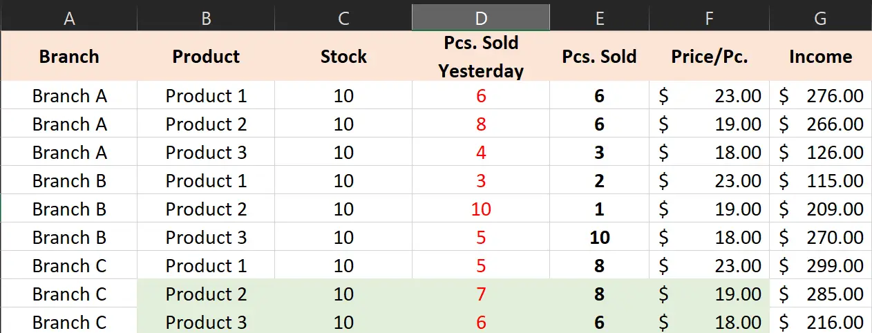
- In this case we will know the sale of product 1, therefore we will use SUMIF function.
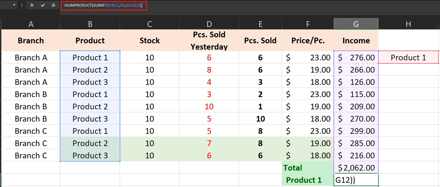
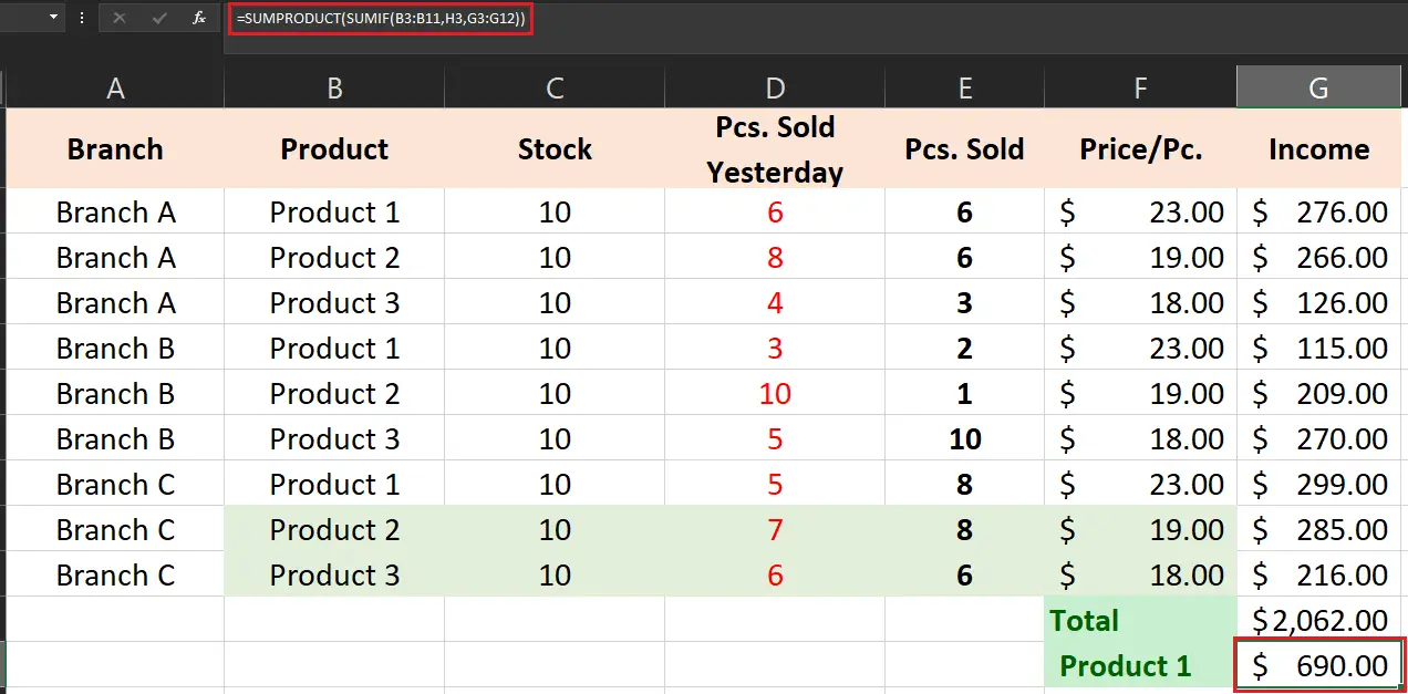
- Now, we will use the SUMPRODUCT formula to calculate the count with multiple criteria. The final output shows the income of product 1 which is 690.
Example 2:
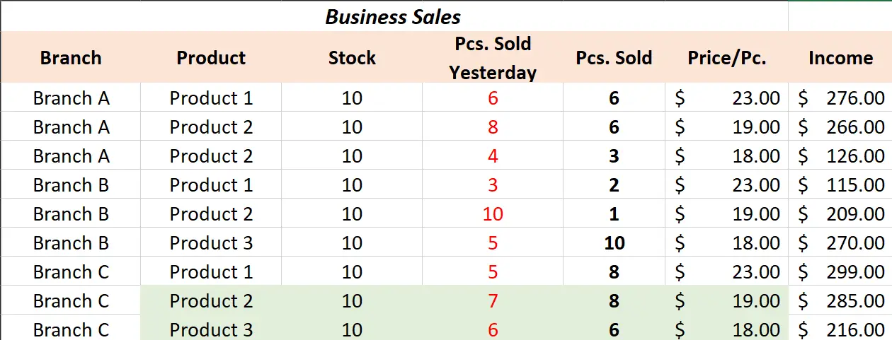
Here is another example where you can see the list of products, branches and products sold. Specifically, we are going to determine how many product 2 are sold in branch A.
Take a look at the figures below for how it works.
- Here is the sample data for this example.
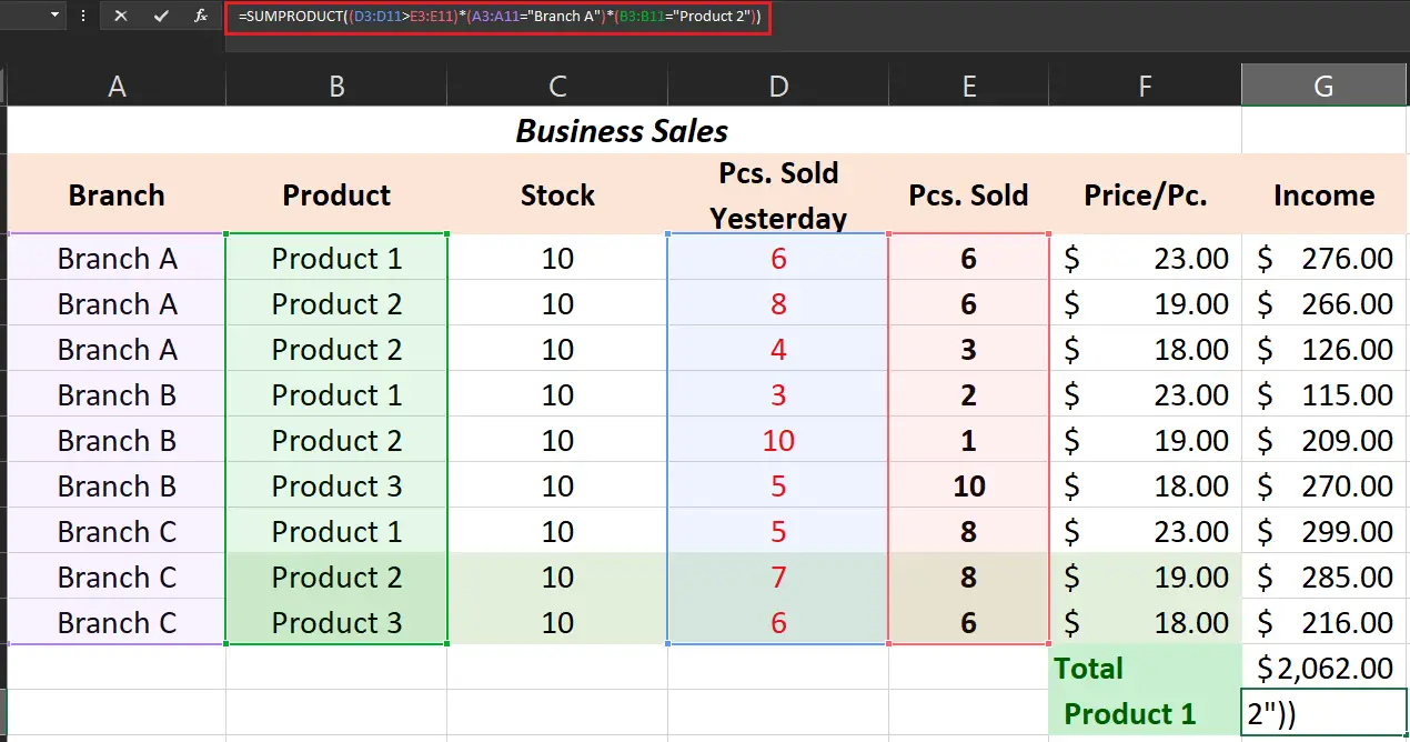
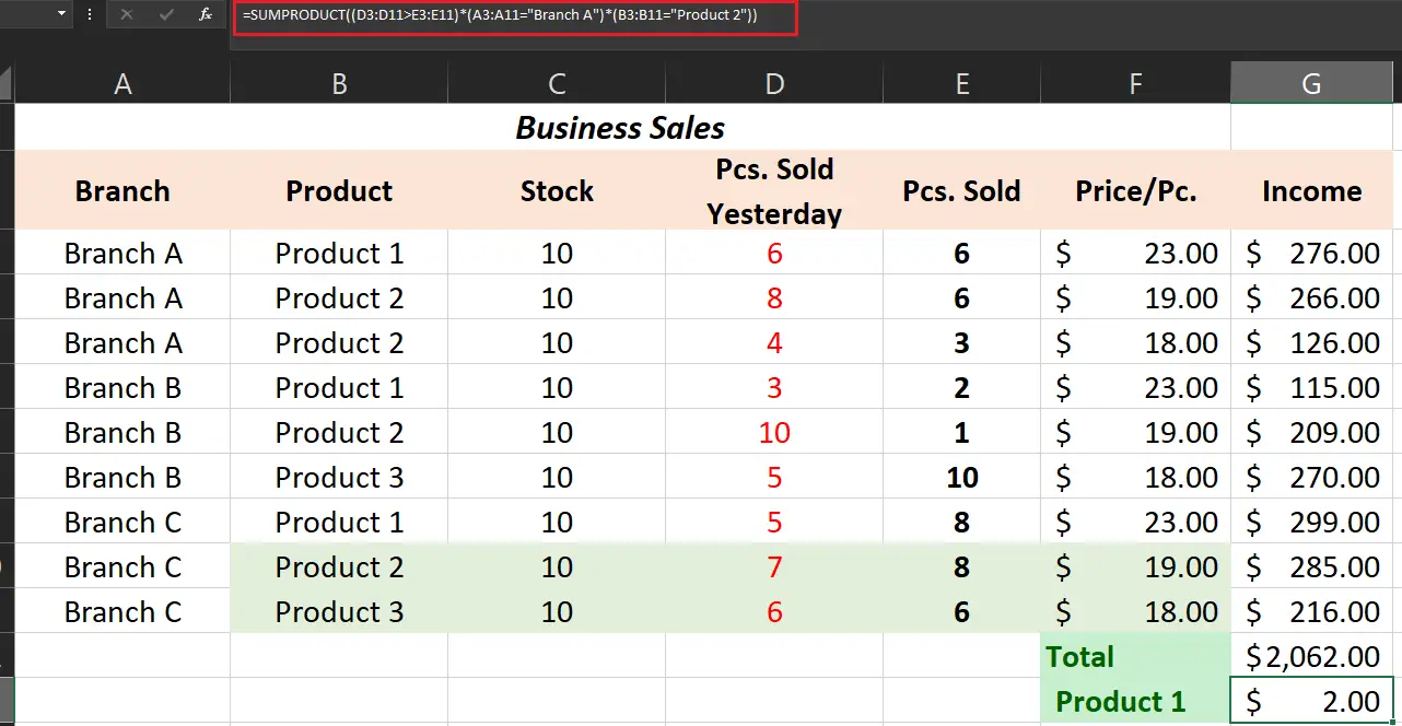
- In this case, we created the formula with the condition where to find pieces sold are greater than the pieces sold. Then this will count the on the branch A and how many product 2 sold on this branch.
- The result of the count of the number of product 2 sold on branch A is 2 which will be the result and displayed below.
What is the difference between SUM and SUMPRODUCT?
Specifically, SUMPRODUCT is adding up the arrays and ranges of cells and returns the product of the total. Meanwhile, the SUM function of Excel sums up the range and arrays with the addition operation.
Conclusion
In conclusion, Excel SUMPRODUCT Formula is very useful as an alternative to SUMIF and COUNTIF other than that it is critical to financial analysts especially in recording and analyzing business sales.
To keep in id here are the things to remember:
- Using SUMPRODUCT your rows and columns should be proportioned otherwise it will return #VALUE! error.
- The non-numeric values read as zeros by the function.
- Use double negative sign or multiple the formula otherwise it will return error.
That’s it! I hope you have gained a lot of learnings and it contributes to your skills in using Microsoft Excel. If you have any suggestions and clarifications feel free to comment below.
Thank you for reading 🙂