In this tutorial, we will see how Count function in Excel is utilized, manipulated, and helpful in doing our worksheet.

As a preview, the excel count function’s role is to return the count values of numbers. Particularly, numbers include percentages, dates, frames, negative numbers and formulas. Otherwise, it will ignore empty cells or value.

Furthermore, we will get deeper into what it is…

What is the Count Function in Excel

The Count Function in Excel yields the counts of numeric values in arguments or value of cells. The count can handle multiple arguments, in the form value1, value2, value3, etc. Additionally, arguments can be individual hardcoded values, cell references, or ranges up to a total of 255 arguments.

All numbers are counted, including negative numbers, percentages, dates, times, fractions, and formulas that return numbers. Empty cells and text values are ignored.

Syntax

=COUNT(value1, [value2], …)

Arguments

value1 – An item, cell reference, or range.
value2 – [optional] An item, cell reference, or range.

Return value

Count of numeric values

What does the Count Function do in Excel

This excel function Count does counts the values of a range of cells that is not empty. Particularly, it uses the following syntax:

=COUNTA(value1,[value2],…)

Additionally, the values involved can be any range too. For instance, A1:A44.

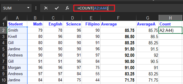
As shown below, =COUNTA(A2: A44) counts cell with numeric data(non-empty cells) in the range, therefore the result is zero because the range is string characters. As you can see, it ignores text values.

Furthermore, the COUNT function counts numeric values and ignores text values see these example function formulas:

Function	Return Value
=COUNT(1,2,3, 4, 5)	Returns 5
=COUNT(2,”b”,”c”)	Returns 1
=COUNT(“book”,110,150,125, 130, “Green”)	Returns 4

In addition to this, the COUNT function is used to count the range. For example, to count numeric values in the range A1:A44:

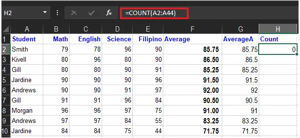
=COUNT(A1:A44) count numbers in A1:A44. It returns 0 because of the range contains text values.

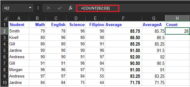
=COUNT(B2:E8) It returns 28. Thus it is made to count numbers in a set range of cells.

The COUNTA function works like the COUNT function, but COUNTA includes numbers and text in the count.

How to use Count Function in Excel

Time needed: 5 minutes

To understand the uses of this function, let us consider a few examples:

Select a cell
Type =COUNT

Double-click the COUNT command
Select a range
Hit enter and you will see the result.

How Do You Use COUNTIF?

The COUNTIF function counts cells that match specific criteria.

The syntax is as follows:

=COUNTIF(range,criteria)

Usage:

COUNTIF can be used to match the criterion with a string.

The two arguments here are:

Range -is a range of cells specified in the formula.
Criteria- a condition on the function. For example: “<80”, A2
This function works on the specified range, counting the cells that match the criteria or condition.

For example:

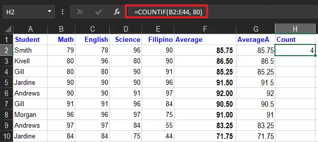
We are using the formula =COUNTIF(B2: E44, 80) to check how many grades match “80”.

Moreover, COUNTIF can be used to count cells with text. Consequently, countif function can also be used to count cells with text values, using wildcard symbols and conditions. So, the (*) asterisk is the symbol used to find wildcards or numbers with any characters.

For instance, =COUNTIF(D2: E12,”*”) will execute and count cells with text.

NOTE: Here, the asterisk symbol helps find cells with any sequence of leading or trailing characters. Thus, this does not apply to boolean values.

COUNTIF can be used to count cells with the help of logical operators: Greater than, equal to, or less than.

For example:

Also, you can use the following logical operations.

Logical operation	Formula Example	Description
Less than “<”	=COUNTIF(F1:F44,”<80”)	Count if the values in cells are lesser than 80
Less than or equal to “<=”	=COUNTIF(F1:F44,”<=75”)	Count if the values in cells are lesser than or equal to 75
Greater than “>”	=COUNTIF(F1:F44,”>90”)	Count if the values in cells are greater than 90
Greater than or equal to “>=”	=COUNTIF(F1:F44,”>=95”)	This Count if the values in cells are greater than or equal to 95
Equal to “=”	=COUNTIF(F1:F44,”=79”)	Count if the values in cells are equal to 79
Not equal to “!=”	=COUNTIF(F1:F44,”<>85”)	Count if the values in cells are not equal to 85

Remember: The criteria MUST be specified within quotes.

How Do You Use COUNTIFS?

The COUNTIF function is a plural co-equal of Countif function, but it calculates multiple criteria of the count cells. So here is the formula syntax for using this function.

=COUNTIFS(range1, criteria1,[range2, criteria2]…)

The syntax implies that range1 is for criteria1 and range2 maps the criteria2 and so on. While using this syntax range1 and criteria1 are the most required arguments while the proceeding is optional, rest in square brackets.

Range1 will be the range of cells to which the first condition (criteria1) will be applied.
Criteria1 defines the condition for the function that will work on Range1. The criteria can be any number, string, or expression, or it can also be a cell reference. For example, “>=75”, ”Smith” or A2.
Similarly, [range2, criteria2] defines another set of range and their respective criteria to be met. They follow an ‘AND’ logic.

Summary

In summary, We hope this article has given you a strong understanding of how various functions are used to COUNT in Excel. The function may seem to perform simple calculations. But when you combine them with other Excel functions, you will be amazed by how powerful Excel is in getting meaning out of enormous datasets.

Do you have any questions related to this article? If so, please mention it in the comments section.

How To Use Count Function In Excel in Simple Way