This tutorial will demonstrate how to add error bars in excel. Also, how to create error bars, how to custom and make individually. Along with, the definitions and figures before proceeding on the guide to make error bars for better learning.

Further, adding error bars into Excel spreadsheets requires only a handful of steps and basic Excel knowledge.

So let’s get started…

What is error bars in Excel?

Online Bookstore Management System in Django with Source Code | Free Django Project with Source Code

Excel error bars are tools that can demonstrate the distance of the reported values from the actual value presented. It is also a useful tool for representing data variability and measurement accuracy.

Further Error bars in Excel can be input in 2-D bar, column, line and area graph, XY (scatter) plot, and bubble chart. Thus, it can be inserted in scatter plot and bubble chart wherin vertical and horizontal error bars will shown.

Correspondingly, error bars can be able to put as percentage, standard error, standard deviation or even fixed value. Another thing is it can able custom error amount thus supply individual value for each error bar.

In Excel, these are the three error bars used by statistical expert:

Percentage: This error bar calculates the percentage of error range shown and basic percentage error on both positive and negative sides. The default percentage is 5%.
Standard error: This error bar displays the standard error amount of all values, average or mean, and determines the sample mean deviations from the population mean.

Standard deviation: This display the standard deviation of all values. The measurement shows how close a sample average remains to the population mean.

Note, you can add one or more error bar nin the chart your are making. It’s the same process of basic insertion in order to minimize confusion.

How to add standard error bars in excel

Now, let’s know how add standard error bars in Excel, 2023 or higher are capable add error bars. Thus it is quick and straighthforward.

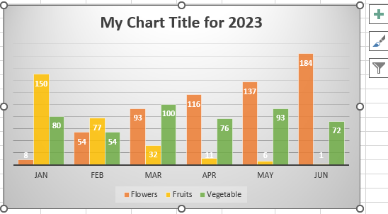
In your chart, Click anywhere.
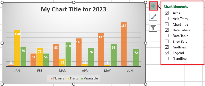
In the right of the graph, Click the chart element button.
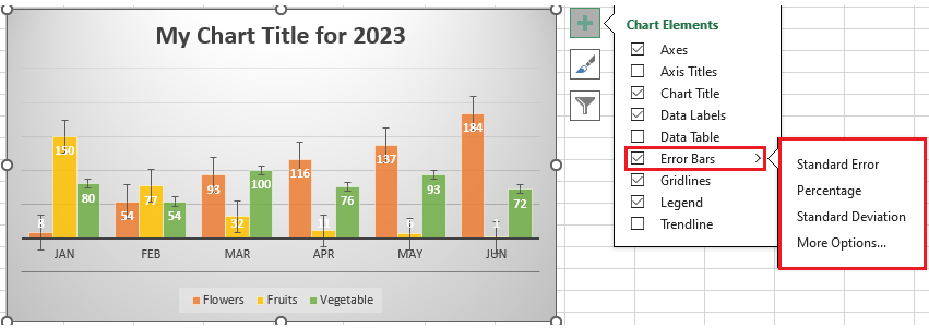
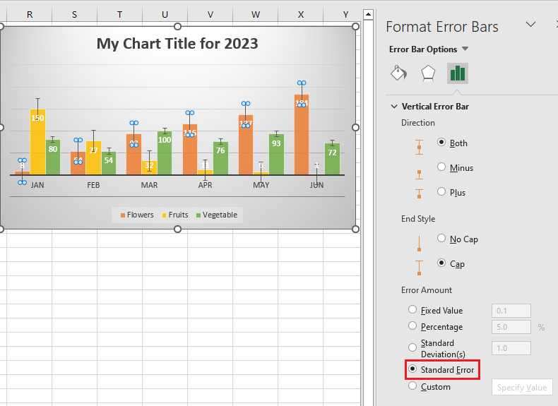
On the Error bars, Click the arrow next to it and select the desired error.

— Standard Error: This value represents the average error for all values in the dataset.
— Percentage: Calculates the percentage error range and amount for each value.
— Standard Deviation: This shows the standard deviation for each value.

Inserting error bars in excel can simply be done by selecting the Error Bars box without picking any option. The standard error bars will be inserted by default.

If you pick More Option opens the format error bars pane which you can:

— Set your own amounts for fixed value, percentage and standard deviation error bars.
— Choose the direction (positive, negative, or both) and end style (cap, no cap).
— Make custom error bars based on your own values.
— Change the appearance of error bars.
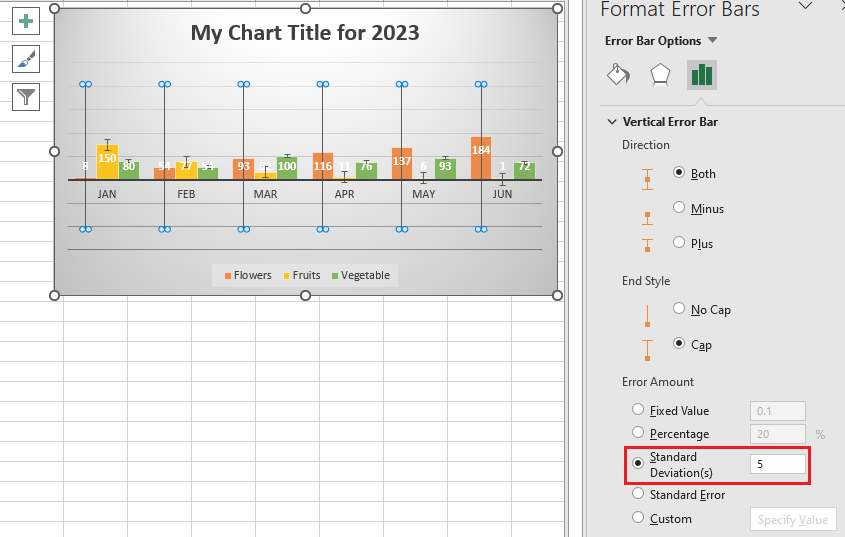
As an example, let’s add 5 error bars to our chart. For this, select stantadard deviation and type 5 in the entry box:

How to add individual error bars in excel

In adding individual error bars in Excel it requires basic Excel calculation or editing menus in excel graphs or charts, or woeksheet.

Follow the steps below on how to complete this tasks.

Spot any location in your chart by clicking anywhere on it. Then the three-icon option will appear.
Click the plus sign–Chart Element icon–.

When the option appears click — Error bars — then click the black triangle icon.
Select ‘More Options’.
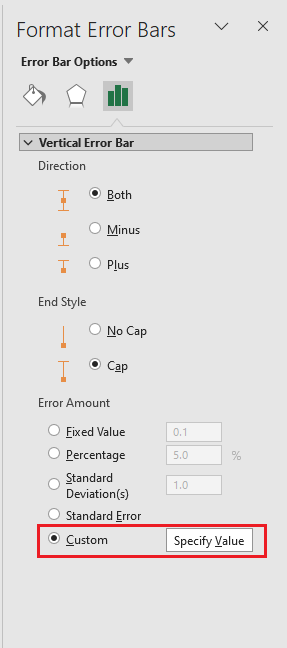
In the Format Error Bars pane, Check the Custom box and click on — Specify Value — button.

Afterward, in the Custom Error Bars dialogue box, delete the contents of the — Positive Error Value box— position the mouse pointer in the box —click the Collapse Dialog icon–, then select a range in your worksheet.
Do the same to Negative Error Value. However, if you don’t want to include negative error bars, Input 0.
Lastly, click the OK button.

How to modify error bars in Excel

You can also change the appearance of your existing error bars, just follow the steps below:

Go to the Format Error Bars pane by doing these steps:
- First Click the Chart Elements button > Error Bars > More Options…
- Right-click error bars and select Format Error Bars from the context menu.
- Double-click the error bars in your chart.
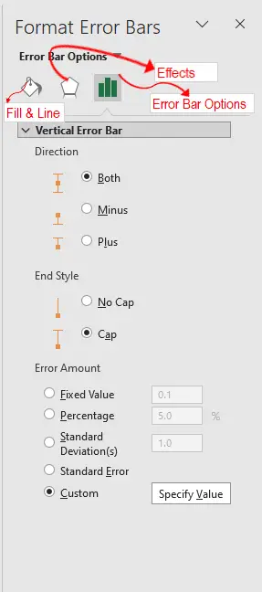
To change type, direction and end style of the error bars, switch to the Options tab.

To change the color, transparency, width, cap, join and arrow type, go to the Fill & Line tab (the first one).

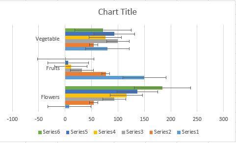
How to add horizontal error bars in Excel?

So far, we’ve only seen vertical error bars. Which are the most frequently used in Excel charting (and can be used with column charts, line charts, area charts, scatter charts).

As you have seen on the error bars above it’s all error bars. Wherein it is most frequently used in charting — with column charts, line charts, area charts, scatter charts– data or spreadsheets.

Meanwhile we can also used horizontal error bars. Thus can use in both bar charts and scatters charts.

Here’s an example of how we plotted data into a bar chart.

Conclusion

To sum up tracking possible errors in data in the worksheet are efficient in improving data analysis. Using this tool gives the audience a better understanding and minimizes data confusion wherein it highlights concerns present in the data.

We finish the guide how to add error bars in Excel. If you have any clarification about this or any other Excel feature, let us know in the comments. We are always happy to help.

How To Add Error Bars In Excel Simple Tutorial