How To Get Average Function In Excel With Examples

In this tutorial, we will now proceed on how to calculate averages’ function in Excel with examples and explanations which make you understand easily.

Excel Average Function

The Excel Average Function is used to calculate the average of numbers, distribution, list of numbers, or a typical range value of numbers. In addition to this, the arithmetic mean is the universal average which is accepted.

Furthermore…

Executing this function you just need to add all the number list or group of numbers and divide it by the total numbers of the list.

Moreover, it can take up to 255 arguments individually, which includes numbers, cell references, ranges, arrays, and constants. Empty cells and cells that contain text or logical values are ignored. However, zero (0) values are included. You can ignore zero (0) values with the AVERAGEIFS function.

The AVERAGE function will ignore logical values and numbers entered as text. If you need to include these values in the average, see the AVERAGEA function.

Consequently, if the values of the AVERAGE contain an error, returns the average error. Otherwise use the AGGREGATE function to ignore errors.

Excel Average Example

In this example Excel average will use on one argument.

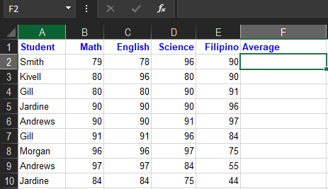
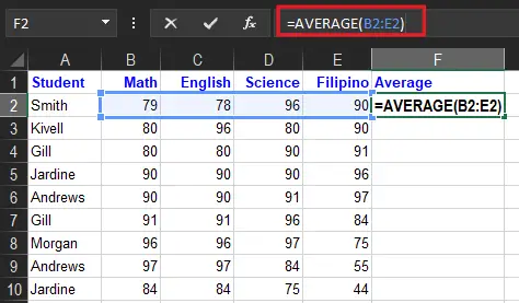
• First, type your sample data in your worksheet. In our example, we get the average of the students.
  • 
• In cell F2, type the average formula to get the average of the grades. =AVERAGE(B2:E2)  
  • 
• Press the Enter key, to complete the formula.
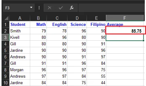
• The result will be 85.75, the average number of cells containing numbers. To quickly get the average of the rest of the cells just double-click the green square and you are done!

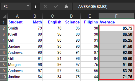
Note: Cells that contain text will not be calculated as well as empty cells.

For your information, there are various average functions in Excel, and there are different methods of how these functions calculate. Therefore below are the following averages that you will learn in this topic.

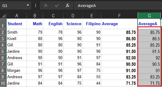
AVERAGEA

AverageA function carries from the average function as it calculates the logical value where the true or false thus the value as text whereas the average skips the values during the calculation. It was introduced in Microsoft Excel 2017 hence it is not available on older versions.

The syntax of this is similar to the average function:

=AVERAGEA(value1, [value2],…)

Instead of exact values, a range of cell or cell references is used. The logic of this AverageA considers values of text as zero while the logical value of true is 1. On the other hand, False is considered as 0 also.

Now let us compare the figure below what is the difference between the average result from the above example to the result of AverageA functions.

Example:

AVERAGEIF

If you want to get the average with specific or multiple criteria the AverageIf function of Microsoft Excel is the best way to do it. Definitely, it looks at the specific range along with the condition, consequently finding the arithmetic mean of the cells which meet the condition.

The syntax of the AVERAGEIF function is:

=AVERAGEIF(range,criteria,[average_range])

Arguments:

• Range: It is the location where we can find cells that meet the criteria.
• Criteria: are the value or expressions that Excel looks within the range.
• Average_range: is an optional argument. This is the range of cells where the values the averaged located. If the average_range is omitted, the range is used.

AVERAGEIF Example

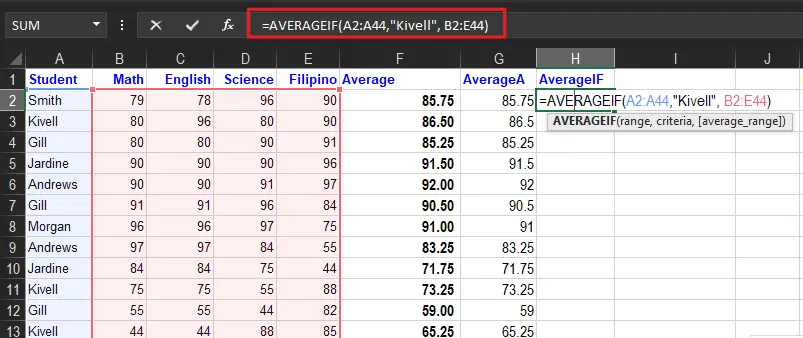
In Excel, to calculate the average of the numbers for cells that meet specific criteria use the averageif function. In this example, only the Kivell average will be computed.

1. Select the cell in which you want to see the average. Here will be placed in cell H2.
2. Type an equal sign (=) to start the formula.
3. Type:   AVERAGEIF(
4. Select the cells that contain the values to check for the criterion. In this example, cells A2:A44 will be checked
5. Type a comma to separate the arguments
6. Type the criterion. In this example, you’re checking for text, so type the word in double quotes:   “Kivell”
   Note: upper and lower case are treated equally
7. Type a comma to separate the arguments
8. Select the cells that contain the values to average. In this example, cells B2:B44 contain the values
9. Type a closing bracket
   The completed formula is: =AVERAGEIF(A2:A44,”Kivell”,B2:B44)
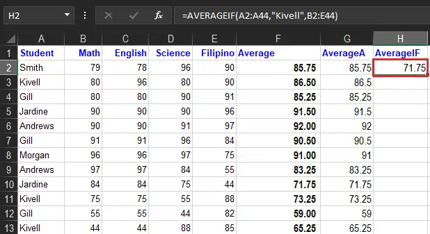
10. Press the Enter key to complete the entry
11. The result will be 71.75, of the values of the average cell for rows that contain “Kivell”.

How to Calculate Weighted Average in Excel

In this case, to compute weighted average in Excel, use the SUMPRODUCT and SUM functions with the formula:

=SUMPRODUCT(X:X,X:X)/SUM(X:X)

Apparently, this formula works when you multiply each value by its weight along with the values. Then, you divide the SUMPRODUCT but the sum of the weights for your weighted average.

Here’s how you do it.

1. Enter your data into a spreadsheet then add a column containing the weight for each data point.

2. Type =SUMPRODUCT to start the formula and enter the values.

3. Click enter to get your results.

Summary

In conclusion, we learned that average in Excel is an acceptable arithmetic mean, thus it does these things:

• AVERAGE can handle up to 255 total arguments.
• You can use the status bar to see a quick average without a formula.
• AVERAGE automatically ignores blank cells and cells with text values.
• AVERAGE includes zero values. Use AVERAGEIF or AVERAGEIFS to ignore zero values.
• Arguments can be supplied as constants, ranges, named ranges, or cell references.