
This tutorial will elaborate the Excel Match function along with examples and how to use it. Moreover, this will helps in your skill in analyzing and lookup and matching data.
Basically based on our prior article there are a lot of lookup functions. These functions are really a great help in finding a certain value in a range of cells. Hence Match function is one of them.
Furthermore, it identifies the relative position of an item in a range of cells. Nevertheless, the match function can do much more than its pure essence.
What is match function in excel
The match function in excel finds the position of the value in a range, row, column, table, or array. Thus, it supports the approximate match, exact match and for the partial match the wildcards(*,?). Usually, the Match function is conjoined with the INDEX function in retrieving value or matched position.
Syntax
=MATCH(lookup_value, lookup_array, [match_type])
Arguments
- lookup_value – The value you find to match in lookup_array.
- lookup_array – A range of cells or an array reference.
- match_type -It is optional 1 = exact or next smallest (default), 0 = exact match, -1 = exact or next largest.
Return Value
Returns the number representing the position of lookup_array.
Example of Match Function:
For a clearer understanding of the match function, here is the basic computation where based on the name of students and their grades in another column, sort it from largest to smallest. This time let’s find where a specific student (andri) is in the position.
Here’s the formula:
=MATCH("andri", A2:A20, 0)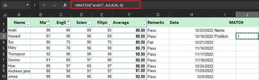
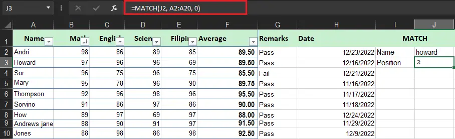
Actually, you can put your lookup value on an empty cell and make it your reference with your formula in our case, it is on [ J2 ].
=MATCH(J2, A2:A20, 0)
Match type Function In excel Information
The argument match type is optional, but if not provided by default set as 1. Thus, sometimes it is an approximate match when the match type is 1 or -1. However, keep in mind that MATCH will find an exact match with all match types, as noted in the table below:
| Match type | Behavior | Details |
|---|---|---|
| 1 | Approximate | This behavior finds the largest, less than, or equal value to lookup. Take note the lookup array required the ascending order. |
| 0 | Exact | Match function searches for the first value equal to the lookup value. The lookup array does not need to be sorted. |
| -1 | Approximate | When the function can’t find the exact match it will find the smallest value, greater than or equal to the lookup value. The lookup array must be sorted in descending order. |
| Approximate | When match type argument is omitted, it defaults to 1 with behavior as described overhead. |
Take note if you want an exact match set the match type to zero(0). The drawback of the default setting of 1 it can cause MATCH to return results that “look normal” hence it’s incorrect. Explicitly providing a value for match_type, is a good reminder of what behavior is expected.
What Does The Match Function Do In Excel
Basically, as we noticed MATCH in excel is simple though like other any other function it has specificities that require a few which should be aware of:
- The match function is not case-sensitive, which means it doesn’t matter if it is lowercase or uppercase when dealing with the text values
- The match function does not return the value itself but rather returns the relative position of the lookup value.
- The first value is returned when the lookup array contains several values.
- #N/A error is returned if the lookup value is not found in a lookup array.
how to use the match function in excel
This time let’s explain the formula that goes beyond the basics of match function, now that you know how it works.
Wildcard for Partial Match
As one of the capabilities of Match function is to accommodate wildcard characters. Let’s understand first these characters:
- Question mark (?) – replaces any single character
- Asterisk (*) – replaces any sequence of characters
Importantly when using wildcard use match_type set to 0 in your MATCH formulas.
A match formula is a great help if you want to look up value whereas not the whole text string but some part of it. Therefore we are going to provide her with some examples that will illustrate this formula.
Assuming you are going to look up the list of student names and grades however you cannot remember the whole name, but a few characters of it.
Considering the student names are in the range A2:A20, and you are searching for a name that begins with “jo”, the formula goes as follows:
=MATCH("jo*", A2:A20,0)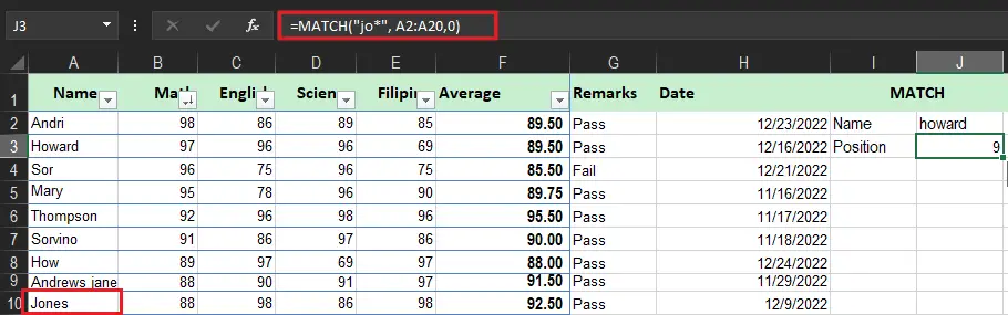
To make our Match formula more versatile, you can type the lookup value in some cell (J2 in this instance), and concatenate that cell with the wildcard character, like this:
=MATCH(J2&"*", A2:A20,0)
As shown in the screenshot below, the formula returns 10, which is the position of “Jones”:
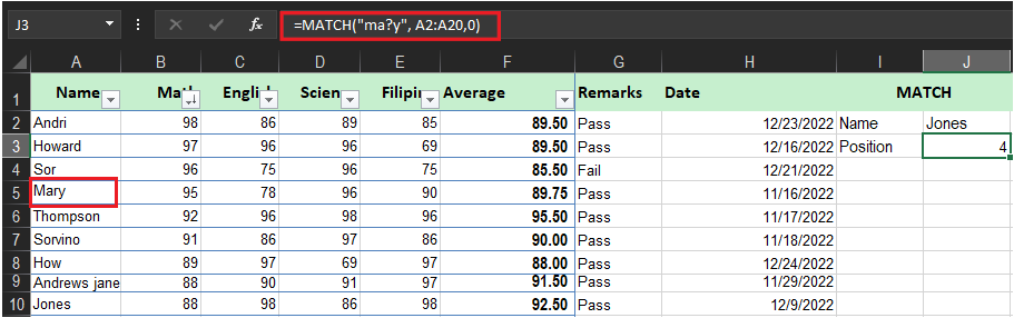
=MATCH("ma?y", A2:A20,0)The above formula will match the name “Mary” and rerun its relative position, which is 5.
Exact match
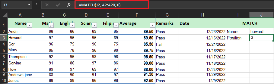
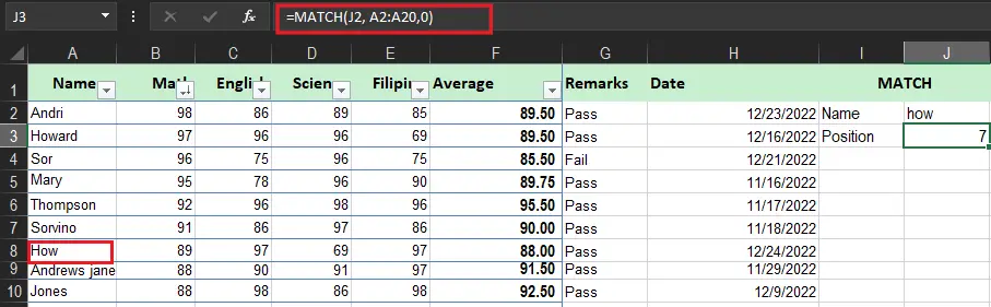
When the match type is set to zero, MATCH performs an exact match. In the example below, the formula in J2 is:
=MATCH(J2, A2:A20,0)
In the formula above, the lookup value comes from cell J2. If the lookup value is hardcoded into the formula, it must be enclosed in double quotes (“”), since it is a text value:
=MATCH("Sor", A2:A20,0)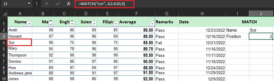
Approximate match
In using match type set to 1 it will execute an approximate match on values sorted A-Z, largest to less than value or equal to the lookup value. For instance, the formula in J2 is :
=MATCH(J2,A2:A20,1)
Case-sensitive MATCH formula
Often times in the beginning that this function is not case sensitive, it does not vary whether it is lower case or uppercase text string. However, if you want this function to be case-sensitive, the MATCH function allows a combination of EXACT functions to execute this function exactly.
Generally, here is the formula to be case-sensitive in matching your data.
=MATCH(TRUE, EXACT(lookup array, lookup value), 0)
The arguments work with the following:
- The EXACT function compares the lookup value from the lookup array, hence if the compared cells are exactly equal it will return TRUE others it will return false.
- The MATCH function compares TRUE (which is its lookup_value ) with each value in the array returned by EXACT, and returns the position of the first match.
- Take note if it is an array formula Press CTRL=SHIFT+Enter to complete the formula.
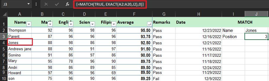
Assuming your lookup value is in cell E1 and the lookup array is A2:A20, the formula is as follows:
=MATCH(TRUE, EXACT(A2:A20,J2),0)
Conclusion
In conclusion, we compete explained the Excel match function which is a really great help in finding a certain value in a range of cells.
Furthermore, it identifies the relative position of an item in a range of cells. Nevertheless, the match function can do much more than its pure essence.
Thank you for reading!

Glay Eliver
Programmer & Technical Writer at PIES IT Solution
Glay Eliver is a programmer and writer at PIES IT Solution, author of over 600 tutorials at itsourcecode.com. Specializes in JavaScript tutorials, Microsoft Office how-tos (Excel, Word, PowerPoint), and Python error debugging covering ImportError, TypeError, AttributeError, ModuleNotFoundError, and JavaScript ReferenceError. Authored several of the site’s highest-traffic Excel and MS Office reference articles.
Expertise: JavaScript · MS Excel · MS Word · MS PowerPoint · Python · Python ImportError · Python TypeError · Python AttributeError · ModuleNotFoundError · JavaScript ReferenceError · Pygame · View all posts by Glay Eliver →