This tutorial will discuss how VLOOKUP function in excel is used. We will cover steps and guides, examples wherein figures are provided, risks and common problems faced in using VLOOKUP function.

Truly, we can not deny the fact that Microsoft Excel is a helpful and powerful tool for managing data, analysis and more. Even today a lot of organizations used it in performing tasks.

Further, Excel provides an extensive function that can make our work easier, especially in looking for specific data vertically across spreadsheets. So VLOOKUP function is one of these. Thus, it possesses a lot of good qualities.

Therefore let’s proceed to explore, and understand what exactly VLOOKUP in Excel is.

What is a Vlookup in Excel

VLOOKUP in Excel literally stands for Vertical Lookup. As the name itself, it is used to look up vertically by searching specific values across your worksheet. In other words, it will search for the value in a column, so that it will return the value from another column on the same row.

It may sound complicated but if you already know how to use it and understand the syntax you’ll realize it’s easier and more beneficial tool.

So here is the syntax of VLOOKUP:

VLOOKUP (lookup_value, table_array, col_index_num, [range_lookup])

Where…

lookup_value: This is the value to look for in our data.
table_array: This is the range of vertical data placed to look inside.
col_index_number: it is the column number that needs to return the value.
range_lookup: This consist of two option. FALSE if looking for an exact match and TRUE when looking for an approximate match.

How to use excel Vlookup

Here is a simple step-by-step guide on how to use Excel Vlookup.

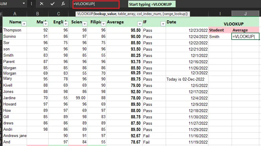
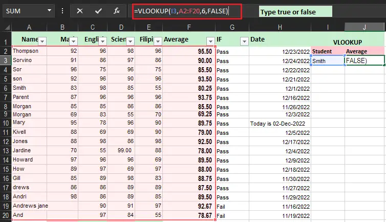
Choose a cell to perform your formula. In our case, cell J3.
Start typing =VLOOKUP.
Double-click the VLOOKUP command
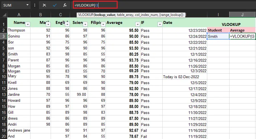
Chose the cell where the looking value will be entered. In our instance i3.
Type comma(,)
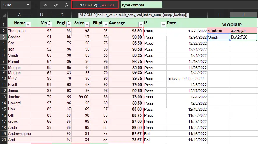
Specify table range. In our case A2:F20.
Type comma (,)
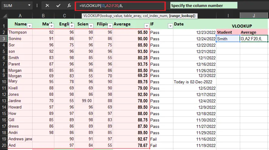
Specify and type the number of the column, it is counted from the left. In our case (6).
Type if the range to look up is True or False.
Press Enter.
You can change and enter value in the cell selected for the Lookup_value.

Excel Vlookup Example

Function of Vlookup in Excel using column number and Exact Match

When using VLOOKUP based on the number of columns starting from the left, you will assume those columns (table array) are numbered. So in yielding the value from provided column, input the column_index_num. For instance, the column index to retrieve the average below is 6:

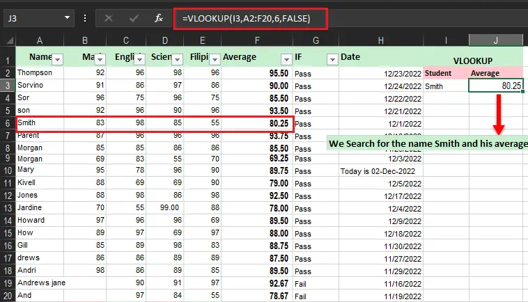
Meanwhile, you can look up columns 3, 4, and 5 all you have to do only change column_index_num. Moreover, we use False for range_lookup to get the exact match result. Examine and try the given examples below.

=VLOOKUP(I3,A2:F20,5,FALSE) // Filipino
=VLOOKUP(I3,A2:F20,4,FALSE) //Science
=VLOOKUP(I3,A2:F20,3,FALSE) // English

Reminder: In certain scenarios, we usually use an absolute reference to prevent varying of formulas when copied or moved. Just like this; I3 ($I$3) and A2:F20 ($A$2:$F$20).

Approximate Match Using VLOOKUP

So we have here the example where we’ll be using VLOOKUP to find an approximate match of the grades of the students. Moreover, we use this because in most cases an exact match cannot be found.

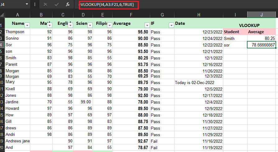
First, have your input your data, and specify your lookup value. Here, we will look up the name of the student Son.
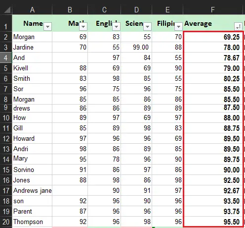
Next, go to the filter and sort option select then select the filter button. After you click on the filter option, you will see the filter buttons enabled on your column headers.
Filter the average details in ascending order. Click on OK.

This time enter your formula VLOOKUP where the first argument is your lookup value, then specify the table range and the column index number, and lastly, put the range to look up which is True.
Press Enter after finishing the formula. The lookup value return in this example is 78.66666667 in the sor.

Multiple criteria Vlookup Function

The VLOOKUP function does not have multiple criteria arguments, but it has a helper column wherein you can be able to combine fields together thus use this as multiple criteria of VLOOKUP. In the sample below, column A is a helper column that concatenates the subject Name and Math with this formula:

=A2&B2 : helper column

VLOOKUP is configured to do the same thing to create a lookup value. The formula in H6 is:

=VLOOKUP(I4&I5,A2:F20,6,0)

Vlookup Function IN Excel Common Problem

Problem	What went wrong
Incorrect Return Value	If using TRUE range_lookup, it requires sorting the first column numerically or alphabetically. Hence, it will return value is something you’re not expecting to be. Alternatively, use FALSE range_lookup.
#N/A	When the result turns #N/A it’s either you are using TRUE range_lookup, then your look_up value is smaller than the smallest value in the table array. Where if the range_lookup is false then the certain value is not found.
#REF!	If the return value is #REF! the col_index_num is greater than the number of columns in table_array.
#VALUE!	If the *table_array* is less than 1, you’ll get the #VALUE! error value.For more information on resolving #VALUE! errors in VLOOKUP, see How to correct a #VALUE! error in the VLOOKUP function.
#NAME?	Usually, this problem means there are missing quotes in the formula. In searching always enclosed names in quotes.
#SPILL!	#SPILL Error particularly means there is implicit on the lookup value, thus using the entire column as reference. However, you can fix this error by anchoring the lookup reference with the @ operator.

Conclusion

To sum up this article How to Use Vlookup Function In Excel With Examples:

This function is not case-sensitive.
It can execute approximate matches.
False and True of range_lookup handle the return value.
- True – approximate
  - returns the closest but less than the look_up value
  - Requires to sort first column in table array.
- False – exact match
  - It does not need to sort column 1.

If you have more clarification and suggest feel free to leave your comment below.

Happy Learning!