
This tutorial describes the whole concept of Excel conditional formatting with examples and different ways to apply it. You will know when and how to utilize this formatting on every version of Excel.
Undoubtedly, excel conditional formatting is very useful when it comes to formatting data that meets a certain condition. Hence will differentiate and highlights important details on your spreadsheets without spending much time.
For beginners users, it seems so complicated and vague to use it. Apparently, this feature is very easy and straightforward you don’t have to be intimidated and uneasy, once you are familiar with this function it will only take a minute to make it.
What is conditional formatting in Excel
Conditional formatting of excel is used in applying format on the data which meets certain criteria or more conditions. Consequently, it automatically applies formatting such as color, icon and data bars, etc.
Furthermore, it highlights and differentiates data from other cells. Besides it is more practical than normal cell formatting because when the data alter the conditional formatted data automatically updates. Hence it’s more flexible and dynamic to use.
Excel conditional formatting is possible to utilize in every cell or on the entire row based on the value of the formatted cell or another cell. Moreover, there are preset tools you can use like Color Scales, Icon sets and Data Bars. In addition, you can also create custom criteria where you like and how you like the selected cells should be highlighted.
Conditional Formatting Excel Location
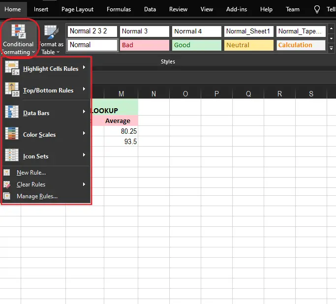
Since excel 2010 throughout 365 version of excel conditional formatting is located in Home Tab >Styles group > Conditional formatting.
After you know where it resides, we’re going to make use of this feature on the worksheet we are working on.

After you know where it resides, we’re going to make use of this feature on the worksheet we are working on. Take note this feature is available in any version of excel you have, so you don.t have any problem with it.
How to use Conditional formatting in Excel
Time needed: 5 minutes
A prerequisite to exploring conditional formatting capabilities is to learn how to use different rule types. Just take note of these two key things on whatever rule you are going to apply:
1. What cells are covered by the rule.
2. What conditions should be met.
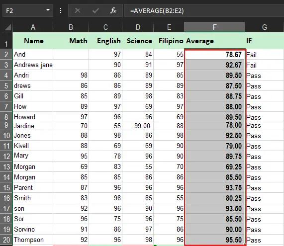
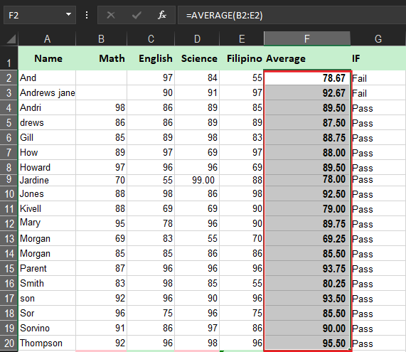
- Select the cells you want to format in your spreadsheet.
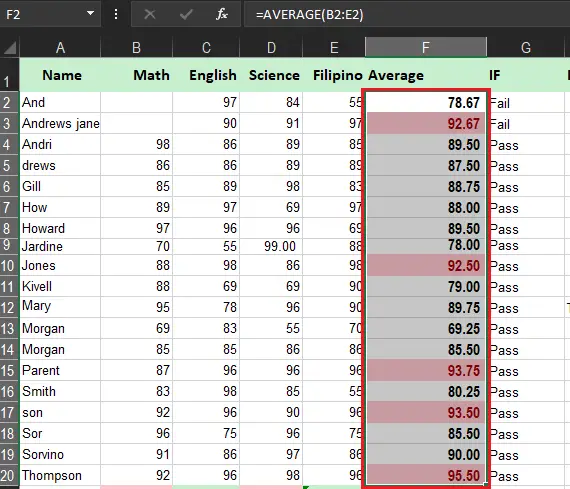
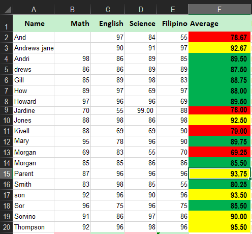
In our sample we select the column Average range F2:F20.

- In your Home tab, click Conditional Formatting, in the Styles group.

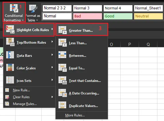
- Select your Rule from the built-in set of Highlight rules fits your perspective.
In our example, we are going to highlight values greater than 90. So we click Highlight Cells Rules>Greater than…

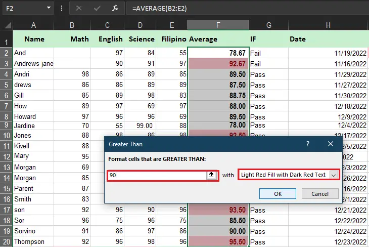
- Enter the value of your rules and select formatting style.
When the dialog box displayed enter the value which in our sample is 90 and then click then select the formatting style (Light Red Fill with Dark Red Text).

- When done, the preview of the formatted formula will display, if you are content with it. Click OK.

Take note can use any other rule depending on your option.
- Greater than or equal to
- Between two values
- Text that contains specific words or characters
- Date occurring in a certain range
- Duplicate values
- Top/bottom N numbers
Conditional Formatting Formula Excel
Take your Excel skills to the next level and use a formula to determine which cells to format. Formulas that apply conditional formatting must evaluate to TRUE or FALSE.
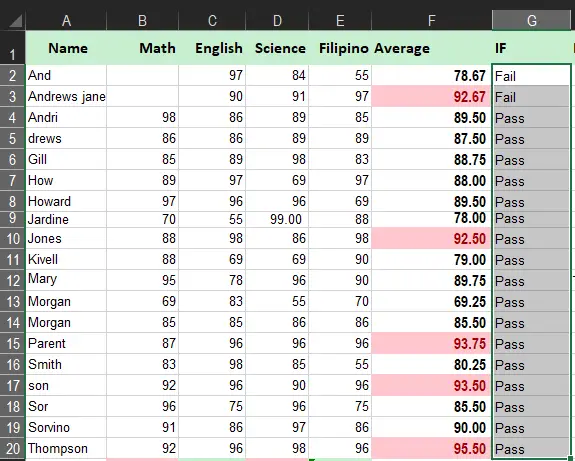
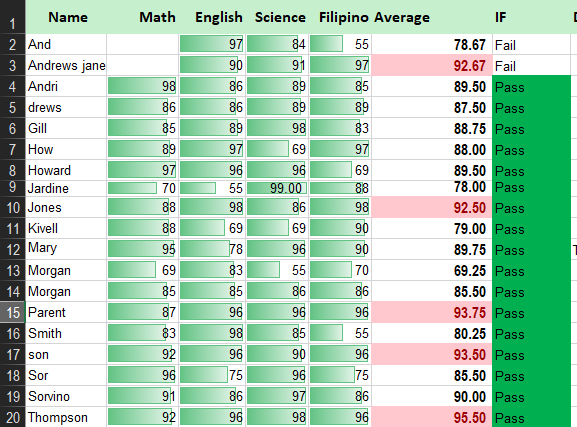
1. Select the range of cells you want to format using the formula. In our sample it’s G2:G20.
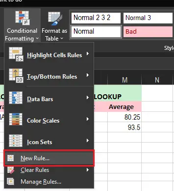
2. On your worksheet Home tab, in the Styles group, click Conditional Formatting. Then when the dropdown list appears, Click New Rule.
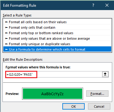
3. Select ‘Use a formula to determine which cells to format‘. Then enter the formula =G2:G20=”PASS”. After you select your preferred formatting rule and Click OK.
4. Then the result of all the pass cells will be highlighted as Green.
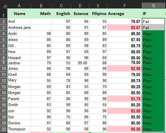
Excel Conditional Formatting Based on Another Cell
Using conditional formatting in your business logic or analysis does not limit you on a single rule only, actually you can add as many as you need.
For instance, you want all grades with a line of nine to be Yellow and a line of 8 to be green thus the line of 7 is red it will work. All you need to do is to specify them correctly.
If the “greater than 99” rule is placed first, then only the yellow formatting will be applied because the other two rules won’t have a chance to be triggered.
To re-arrange the rules, this is what you need to do:
- Select any cell in your dataset covered by the rules.
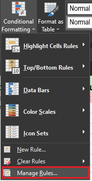
- Open Conditional Formatting then Click Manage Rules… to proceed to Rules Manager.
- Click the rule that needs to be applied first, and then use the upward arrow to move it to the top. Do the same for the second-in-priority rule.
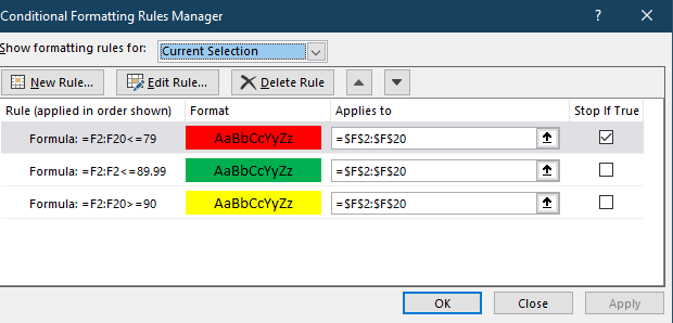
- Select the Stop If True check box next to all but the last rule because you do not want the subsequent rules to be applied when the prior condition is met.
Conditional Formatting Presets
Excel has several conditional formatting presets that will help you quickly apply to your data. Mainly it consists of three categories:
- Data Bars: These horizontal bars are inserted into each cell, likely a bar graph.
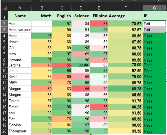
- Color Scales: The color of each cell changes depending on the value. The color of the scale uses two or three gradients. For instance, on the Green-Yellow-Red color scale, the highest values are green, the average values are yellow, and the lowest values are red.
- Icon Sets: It enters a specific icon on the cell based on its value.
Summary
To sum up, this article about excel conditional formatting includes ways where to apply and examples that clarify the usefulness of conditional formatting.
If you have missed our other tutorials you can visit MS Excel tutorial for more.
See you on our next tutorial. Thank you for reading!

Glay Eliver
Programmer & Technical Writer at PIES IT Solution
Glay Eliver is a programmer and writer at PIES IT Solution, author of over 600 tutorials at itsourcecode.com. Specializes in JavaScript tutorials, Microsoft Office how-tos (Excel, Word, PowerPoint), and Python error debugging covering ImportError, TypeError, AttributeError, ModuleNotFoundError, and JavaScript ReferenceError. Authored several of the site’s highest-traffic Excel and MS Office reference articles.
Expertise: JavaScript · MS Excel · MS Word · MS PowerPoint · Python · Python ImportError · Python TypeError · Python AttributeError · ModuleNotFoundError · JavaScript ReferenceError · Pygame · View all posts by Glay Eliver →