
This guide will explain how to merge cells in Excel along with the step-by-step guide along with figures which are provided to acquire a better understanding.
The common purpose of merging cells is for formatting and centering of headings. Therefore this discussion will explain how merging cells in Excel happens. Meanwhile we suggest to avoid using it frequently, particularly if not needed. Alternatively, use center across selection feature.
What is Merging Cells?
Merging cells is a function which can provide uniform formatting in multiple strands of data. This will both merge vertically and horizontally cells range.
By doing that, the spreadsheet displays data in one large cell rather than multiple columns. It makes the spreadsheet look clean and presentable.
How To Merge Two Cells in Excel
As know already that merging cells is combining two or more cells into single large cell. Now let’s look at the steps on how to merge cells in Excel using Windows OS.
- Open Microsoft Office Excel as well as the worksheet with data.
- Highlight the cells or two cells using a mouse by dragging over the cells while holding the left click.
Another way of selecting the desired cells is to determine the starting cell, hold shift and press the right arrow key to select all the adjacent cells.
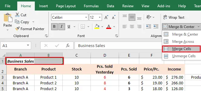
- Find the “Merge” button under the “Home” tab and click on “Merge Cells.”

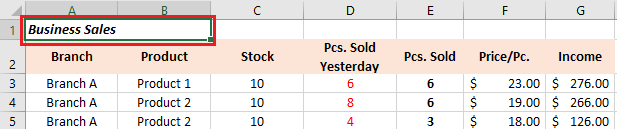
- The three steps are simple, cells A1 and B1 are merged.

Reminder: The process only we did only saves the data in the left cell (in this case, A1). So id the B1 or any data adjacent to them you need to cut and paste data to another place before merging cells so that no data will be lost.
How to Merge Cells Without Losing Data
On the other hand in order to merge cells without losing data we are going to use Concatenate function. For instance, we are going to enter the formula =Concatenate(A1, ” “, B1).
So when we combine the cells A1 and B1 and have a space character as the separator. However, if you don’t want any separator, you can simply leave it out and use the formula =CONCATENATE(A1,B1).
Meanwhile, you can also use commas and semi-colons as other separators.
The result of the CONCATENATE function is on another cell, but if you want it to the cells you wanted to merge just copy and paste the value into the cell.
You can also use the ampersand sign to combine text. For example, you can also use =A1&” “&B1
Center Across Selection
As it mention already merging cells interupts the functions of Excel particularly in creatring financial model. For instance in trying to delete and insert columns across the merged cells and its unable to do.
Nevertheless Excel provides function which the same as merging cells this is Center Across Selection function.
Follow the steps below to perform the action yourself.
- Step 1. Select the cells you want to center using the mouse or hold the Shift key and use the keyboard arrows.
- Step 2. On the Home Ribbon Tab open the Format Cells dialogue box, or just press Ctrl + 1 for the Windows shortcut.
- Step 3. Then click the Alignment tab and then select Center Across Selection.
Note: Make sure to uncheck Merge Cells if it’s already checked.
Conclusion
In conclusion, we learn how to merge cells in excel, along with we learned that if not necessary we should not use merge cells. This is because it can limit some functions to work which is a little bit of hassle in working the task, especially in sorting and filtering data.
However, there are alternatives to use if ever certain circumstances might happen. These are concatenate functions and center across selection feature.
There you have it! you learn how to merge cells.
Thank you for reading 🙂

Glay Eliver
Programmer & Technical Writer at PIES IT Solution
Glay Eliver is a programmer and writer at PIES IT Solution, author of over 600 tutorials at itsourcecode.com. Specializes in JavaScript tutorials, Microsoft Office how-tos (Excel, Word, PowerPoint), and Python error debugging covering ImportError, TypeError, AttributeError, ModuleNotFoundError, and JavaScript ReferenceError. Authored several of the site’s highest-traffic Excel and MS Office reference articles.
Expertise: JavaScript · MS Excel · MS Word · MS PowerPoint · Python · Python ImportError · Python TypeError · Python AttributeError · ModuleNotFoundError · JavaScript ReferenceError · Pygame · View all posts by Glay Eliver →