
In this tutorial, we are plainly going to explain what is SUMIF function in Excel. Along with given examples and guide on how to use it. Given also different scenarios wherein we can use and combine this function.
A good thing about this function is, instead of summing up all ranges of cells you can now sum only those cells you want. Also with specific criteria.
Therefore, if your worksheet requires adding specific criteria this function is very useful. Another good thing about this is it’s available in any version of Excel such as Excel 365, Excel 2021, Excel 2019, Excel 2016, Excel 2013, Excel 2010, Excel 2007, and lower.
Further, if you master this function you will be ready. Hence it will be easy for you to proceed and master more IF functions like SUMIFS, COUNTIF, COUNTIFS, AVERAGEIF, etc.
So let’s begin with what this function is all about…
What is SUMIF Function in Excel?
SUMIF function is an Excel function which sums up cells which have met a single condition or known as criteria. It’s commonly known as conditional SUM. Further, this function is commonly used and can able to sum cells based on dates text values, and numbers.
Syntax
=SUMIF(range, criteria, [sum_range])
Arguments
It consists of three arguments which 2 are required and the rest is optional.
- Range — This is a required argument which is the range of cells to be evaluated.
- Criteria — A required argument and this is a condition required to meet. Additionally, this argument can be supplied by a number, text, date, logical expression or another function.
- Sum_range — an optional argument and this is the range to sum and if omitted the range of cells is summed.
Return Value
The return value is the sum of matching cells.
Things to Remember. When using text as criteria or logical operators it must be enclosed in double quotation marks. Meanwhile using cell reference as criteria does not need to enclose in double quotes, otherwise it will read as text string.
SUMIFS function in Excel Example
And now to utilize the given syntax above, we will give examples which indicate in detailed utilization of SUMIF from basic to advanced:
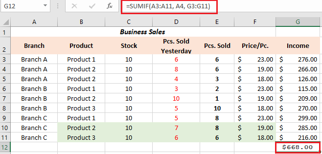
Assumingly, we have data of Business sales in three branches and products. So the goal is to get the total income on a specific branch, Branch A. So to know how it works let’s build a formula based on the syntax given.
So our range argument is the list of Branch (A3:A11).
The Criteria is Branch A or cell A4 and our sum_range is a range of cells G3:G11.
Technically the formula could be like this:
=SUMIF(A3:A11, A4, G3:G11) or =SUMIF(A3:A11, "Branch A", G3:G11)
How to use SUMIF
Since you already know to create basic formula for SUMIF, now we will know how to use SUMIF with other criteria.
SUMIF with logical operators
We can now sum a range of cells with the use of logical operators. Particularly we are going to configure the following in our SUMIF criteria.
- Greater than (>)
- Less than (<)
- Greater than or equal to (>=)
- Less than or equal to (<=)
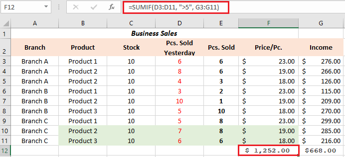
For instance, we have the worksheet of Business Sales and we are going to add the sales of greater than 5 Pcs. sold in yesterday column. To create this condition, put a comparison operator (>) before the number. Then surround the criteria in double quotes (“”):
=SUMIF(D3:D11, ">5", G3:G11)
Whenever the criteria are on another cell, just concatenate the logical operator and cell reference.
=SUMIF(D3:D11, ">"&D9, G3:G11)
In a similar manner, you can sum values smaller than a given number. For this, use the less than (<) operator:
=SUMIF(D3:D11, "<5", G3:G11)
Another scenario is using the equal to logical operator.
Truly using equal to logical operator in sumif formula works in numbers and text. And actually, in doing such criteria it is not required to put an equal sign(=) in the formula.
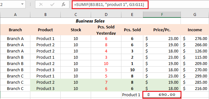
To understand it better, for instance we are going find income of product 1 in all branches, the formula below will do this:
=SUMIF(B3:B11, "product 1", G3:G11) or =SUMIF(B3:B11, "product 1", G3:G11)
In using cell reference in sumif equal to the formula is as follows:
=SUMIF(B3:B11,B3, G3:G11)
Wherein B3:B11 is the list of products and G3:G11 is the list of incomes, thus B3 is the criteria that contain product 1.
Apparently, you can also use equal to in number values. Like for instance to sum up income with 5 pcs sold you can utilize any of the formulas below:
=SUMIF(D3:D11,5, G3:G11)=SUMIF(D3:D11,"=5", G3:G11)=SUMIF(D3:D11,D9, G3:G11)
So aside from equal to we have…
SUM IF not equal to
In sumif not equal to we use the symbol “<>” logical operator. Technically this works in text or number value. However again always put double quotes in text string values.
For instance, we are going to get the income which not product 2, then the formula as follows:
=SUMIF(B3:B11, "<>product 2", G3:G11)
When the criterion is in another cell, concatenate the “not equal to” operator and a cell reference like this:
=SUMIF(B3:B11, "<>" &B4, G3:G11)
SUMIF vs SUMIFS
The SUMIF function is used to return sum of of cell with a single criterion. Meanwhile, SUMIFS function is used to sum range of cells with multiple criteria to meet. Thus criteria to meet is can be numbers, dates or text.
Advanced SUMIF function in Excel
Date
Generally, using DATE function and valid date of another cell is the efficient way in working SUMIF with dates. Take a look at the example formula below:
=SUMIF(B3:B11,"<"&DATE(2023,1,10),C3:C11)=SUMIF(B3:B11,"<"&DATE(2023,1,12),C3:C11)=SUMIF(B3:B11,"<"&E6,C3:C11)
As you can see, on the last formula we concatenate the logical operator to the cell E6 which contains date. However, to use more advanced date function criteria — more than one dates given in month, day or between two dates– you will use SUMIFS function which we will tackle next article.
Wildcards
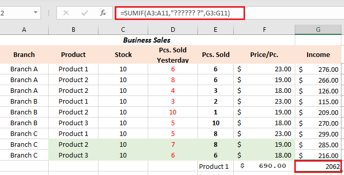
The SUMIF function supports wildcards, as seen in the example below:
=SUMIF(A3:A11,”?????? ?”,G3:G11)
Use tilde (~) escape character to find literal wildcards. For example, to match a literal question mark (?), asterisk(), or tilde (~), add a tilde in front of the wildcard (i.e. ~?, ~, ~~).
Conclusion
As a recap SUMIF function is an effective tool. Definitely use it since you discover how helpful it is especially in certain data that only require a specific cell to sum.
Thank you for reading 🙂

Glay Eliver
Programmer & Technical Writer at PIES IT Solution
Glay Eliver is a programmer and writer at PIES IT Solution, author of over 600 tutorials at itsourcecode.com. Specializes in JavaScript tutorials, Microsoft Office how-tos (Excel, Word, PowerPoint), and Python error debugging covering ImportError, TypeError, AttributeError, ModuleNotFoundError, and JavaScript ReferenceError. Authored several of the site’s highest-traffic Excel and MS Office reference articles.
Expertise: JavaScript · MS Excel · MS Word · MS PowerPoint · Python · Python ImportError · Python TypeError · Python AttributeError · ModuleNotFoundError · JavaScript ReferenceError · Pygame · View all posts by Glay Eliver →