
In this tutorial, we will learn quick analysis tools in Excel as well as how to use it and where we can find this tool.
Fortunately, provides various ways to visualize data however it is hard to determine where to start. Then it where Quick Analysis tool comes in, it permits you to browse a lot of options when you don’t know exactly what you needed.
What is Quick Analysis tool?
Quick Analysis tool helps to format easily your data along with your table, chart, summary formula, sparkline, or highlighted figures with just a few simple steps.
Further, when selecting a range, quick analysis tool will appear on the lower part of the selected data. Once you click it, a variety of options will appear such as charts, sparklines, conditional formatting options, and more.
Additionally, this tool is very dynamic wherein it provides a whole range of data analysis options. It quickly analyzes data it just a click.
Where is Quick Analysis tool
You will be surprised if you search quick analysis tool in the Excel ribbon and you can not find it there.
Apparently, it will only appear whenever you select a range of data. Actually, you can also use keyboard shortcut just press “Ctrl+Q” after selecting a Data range to access it.
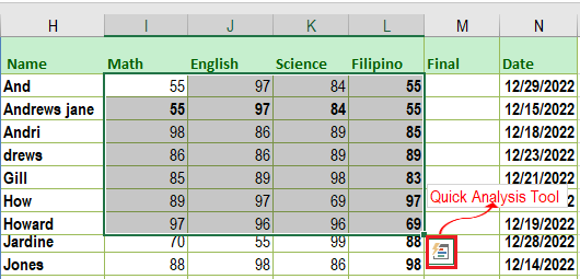
Note: It will not appear if you have selected blank cells or the entire column.
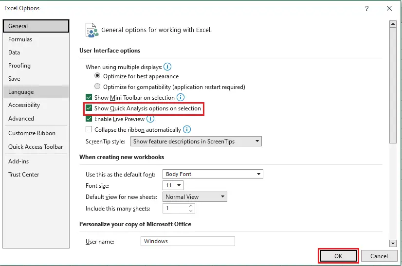
Whenever it does not appear, it might be disabled. Hence, to enable just go to File tab> Options>locate General Tab.
Afterward, under the general tab just check the check box “Show Quick Analysis Options on Selection” to enable the quick analysis tool.
Quick Analysis tool in Excel Mac
Meanwhile, if you are using Mac you just need your keyboard and mouse. Just go to File>Tools>Excel Add-ins. Then in the Add-in box check the Analysis ToolPak check box, and then click OK. The helpful tool and the list of options should open on your screen.
How to use Quick Analysis tool in Excel
Now we will learn this simple example on how to use a quick analysis tool in Excel.
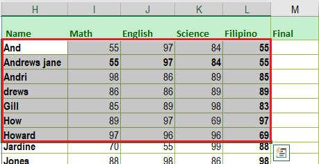
- Select the cell range you want to summarize.
When selecting data range, be careful because the Quick Analysis button will not appear when using the Ctrl key to make multiple selections.

- Click the Quick Analysis button.
- Select the type of analysis tools you want to use.
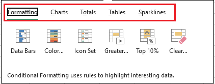
When the analysis tool appears you can select what you prefer to add it could either be the following:
Formatting: It highlights the data with the use of conditional formatting.
Charts: It allows you to create charts with the selected data.
Totals: It can make a common summary formula.
Tables: It will summarize data in a table or PivotTable.
Sparklines: You can create Mini charts placed in single cells.
Conclusion
In conclusion this tutorial about Excel Quick Analysis tool is a dynamic feature which a great help when you don’t know exactly what to do, it suggests options crucial in analyzing data.
So there you have it! We already covered this topic and now you already now know how to quickly add tables, charts, conditional formatting and more.
Thank you for reading.

Glay Eliver
Programmer & Technical Writer at PIES IT Solution
Glay Eliver is a programmer and writer at PIES IT Solution, author of over 600 tutorials at itsourcecode.com. Specializes in JavaScript tutorials, Microsoft Office how-tos (Excel, Word, PowerPoint), and Python error debugging covering ImportError, TypeError, AttributeError, ModuleNotFoundError, and JavaScript ReferenceError. Authored several of the site’s highest-traffic Excel and MS Office reference articles.
Expertise: JavaScript · MS Excel · MS Word · MS PowerPoint · Python · Python ImportError · Python TypeError · Python AttributeError · ModuleNotFoundError · JavaScript ReferenceError · Pygame · View all posts by Glay Eliver →