Excel Index Function Example, Formula, How to Use

This article explains the Excel Index function examples, formulas and how to use it in your worksheet.

What does this index function do in excel? it may sound unimportant but if you learned its functionality it will be a big help in analyzing and presenting your data.

What is the index function in Excel

The index function of excel returns the array or range actual value in a specified number of indexes. It is a versatile and supple function wherein you can be able to retrieve individual values of row or even the entire column.

Further, this function is available in all versions of Microsoft Excel. Using this in your calculations you can determine the actual value of the element when you know the position of the range. Asides from that it can extract an array value of data set.

Here is the syntax of this function:

=INDEX(array, row_num, [col_num], [area_num])

Where the arguments are defined as follows:

• array – A range of cells, or an array constant.
• row_num – The row position in the reference or array.
• col_num – It is optional and it is the position of the column in the array or reference.
• area_num – It is optional thus it should be used as a range in the reference.

Hence, it returns the value of the given location.

Index Function in Excel Basic Usage

As already mentioned, index function extract the value in a given location. We’ll see here the basic usage when the range is a single dimension, either two or three dimensions. However if two or more dimensions you need to include the row and column number.

For example:

1. =INDEX(A2:A20,2)
2. =INDEX(A2:B20,4, 5)

These examples are the basic usage of INDEX function and easy-to-make formula.

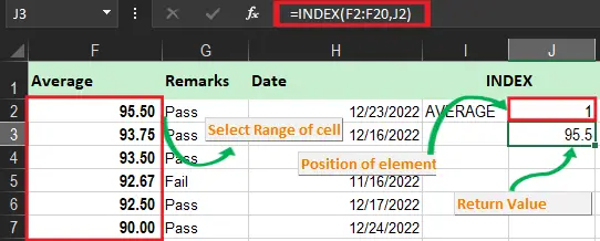
Basically the syntax is =INDEX(range, n) which range is the range of cells and n is the position of the element you want to extract.

So here is the image that shows the result of the formula structure for index.

Now to get the value of the cell across rows and columns, the approach is the same the only thing is row and column numbers must be specified.

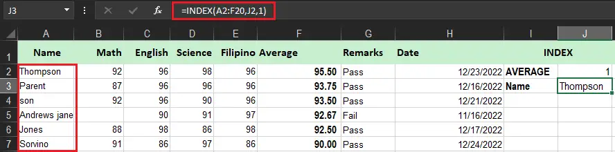
Here now another example to make it clear. This time we will know who is the top 1 according to the average ranking. Take note to sort first the average column from largest to smallest or what suits your requirements.

=INDEX(A2:F20,J2,1)

The formula above returns the name of a person who meets the criteria.

Thus, you can use a cell reference in the row_num and/or column_num arguments to make your formula more versatile, as demonstrated in the screenshot below:

What does Index Function do in Excel

The index function can return values from a range or table in two ways:

An array formula is a way in which you can return the specified array or call. This retrieves the value of an element in table or range of an array determined by the row and column number indexes.

Additionally, use the array form if the first argument to INDEX is an array constant.

In retrieving references with specified cells or array cells use the reference form. This return the reference of the cell at the intersection of a particular row and column. Refer to this syntax if you want this way:

INDEX(reference, row_num, [column_num], [area_num] )

Consequently, if the reference is made up of non-adjacent selections, you can pick the selection to look in.

How do you use INDEX reference in Excel

Using the INDEX reference form these are things to remember:

1. Respectively, the Index formula returns the reference for the entire row and column if the row_num or column_num argument is zero(0).
2. The INDEX formula returns the specified area in the area_num if both row_num and column_num are omitted.
3. The index formula will return #REF! error if not all of the num_argumets refer to a cell of the reference.

How to use the index Formula in Excel

Using INDEX with other functions (SUM, AVERAGE, MAX, MIN)

Based on the basic usage of the Index function it returns value however it is actually a reference that contains value. This time examples will describe the actual nature of Index function.

Since Index function is a reference we use it in the dynamic range. It is confusing right? but it will be clear when we encounter few examples.

For instance in using the formula =Average(B2:B20) which will return the value cells B2: B20. Instead of writing the range directly in the formula, you can replace either B2 or B20, or both, with INDEX functions, like this:

=AVERAGE(B2   : INDEX(B2:B20,2))

The average above shows the formula and yield the same result wherein INDEX function returns to cell B2 (row_num is set to 2, col_num argument omitted). Moreover the discrepancy is the range is the Average/INDEX which is dynamic and once you change the row_num argument in Index the range processed by the AVERAGE function will change and the formula will return a different result.

Apparently, the INDEX formula’s route appears overly complicated, but it does have practical applications, as demonstrated in the following examples.

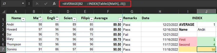
Example 1. Calculate average

Suppose we will get the average of student grades in the math subject. Therefore we will sort the table in Math column from largest to smallest and will utilize the INDEX/Average formula.

=AVERAGE(B2     : INDEX(Table1[Math], J5))

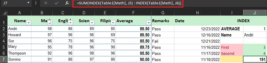
Example 2. Sum items between the specified two items

In case you want to sum items between the specified two items in your formula, you just need to employ two INDEX functions to return the first and the last item you want.

For example, the following formula returns the sum of values in the math column between the two items specified in cells J5 and J6.

=SUM(INDEX(Table1[Math], J5) : INDEX(Table1[Math], J6))

Is INDEX better than VLOOKUP?

How can we tell INDEX is better than VLOOKUP? Well, Vlookup should always begin to look up the value from the left column of a range since it’s incapable to look up to its left common column. Meanwhile, the INDEX and MATCH functions are not functioning that way.

Additionally, INDEX and Match functions are working without distorting the results when a new column is inserted or deleted.

Unfortunately, in Vlookup formulas get broken when columns are deleted or inserted on the data consequently it returns incorrect results.

Hence, Index has these superiorities from Vloolup such as:

• No problem with left lookups
• No limit to the lookup value size
• Sorting is not required, unlike VLOOKUP you have to do always the ascending sorting.

Along with you are able to add or delete new columns without affecting and updating the formula, importantly it does not slow down Excel from multiple lookups.

Refer to this syntax:

=INDEX (column to return a value from, (MATCH (lookup value, column to lookup against, 0))

Conclusion

In conclusion with this topic index function in excel is crucial especially if you are trying to return exact values in that specific position of cells.

Thank you for reading!