
In this article, we will describe the AVERAGEIF function in excel, how we can use it, and how examples help in understanding this topic.
Still, it is the continuation of average function, but before proceeding with the methods and examples, let’s defined first the excel averageIf function.
What is the AVERAGEIF Function?
The AVERAGEIF Function is a statistical function which calculates the average of the range of cells with a true or false condition. Moreover, it is a function that yields according to its specific or multiple criteria. Criteria of this function could be supplied as numbers, strings, or references.
Primarily, AVERAGEIF calculates central tendency, which is the location of the center of a group of numbers in a statistical distribution. This was introduced in Microsoft Excel 2007, hence this is not functional in older versions.
Syntax
=AVERAGEIF(range, criteria, [average_range])
Arguments
- Range – Required. One or more cells to average, including numbers or names, arrays, or references that contain numbers.
- Criteria – Required. The criteria that define which cells are averaged, expressed as a number, expression, cell reference, or text.
- Average_range – Optional. The actual set of cells to average. If omitted, the range is used.
Return Value
A number representing the average.
The condition is referred to as criteria, which can check things like:
- If a number is greater than another number
>. - If a number is smaller than another number
<. - If a number or text is equal to something
=.
Example AVERAGEIF Function
In the example shown the formulas in B2:E10 are as follows:
=AVERAGEIF(F2:F10,"<79") // grade is failed
=AVERAGEIF(F2:F10,">79") // Passed
=AVERAGEIF(F2:F10,">=85",B2:E10) // Add five points
=AVERAGEIF(B2:E:10,">=90",F2:F10) // Add 10 points
| Formula | Description | Result |
| =AVERAGEIF(B2:E2,”<88″) | Average of all grades less than 88. | 78.5 |
| =AVERAGEIF(B3:E3,”<90″) | The average of all student grades values less than 90. | 80 |
| =AVERAGEIF(B4:E4,”<79″) | The average of all student’s grades values less than 79. Because there are 0 property values that meet this condition, the AVERAGEIF function returns the #DIV/0! error because it tries to divide by 0. | #DIV/0! |
| =AVERAGEIF(B2:E5,”>90″,F2:F5) | Average of all commissions with a property value greater than 90. | 82.5 |
How to do an AVERAGEIF Function in Excel
Time needed: 5 minutes
Here is the step-by-step of AveregeIf function in Excel.
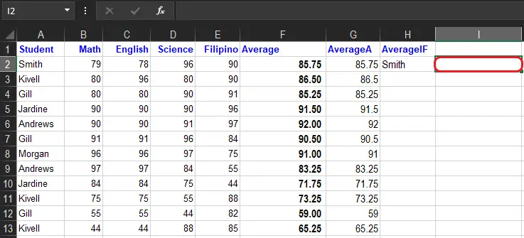
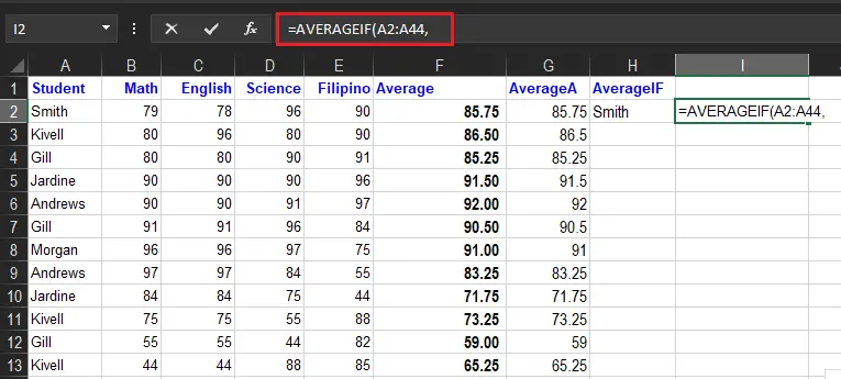
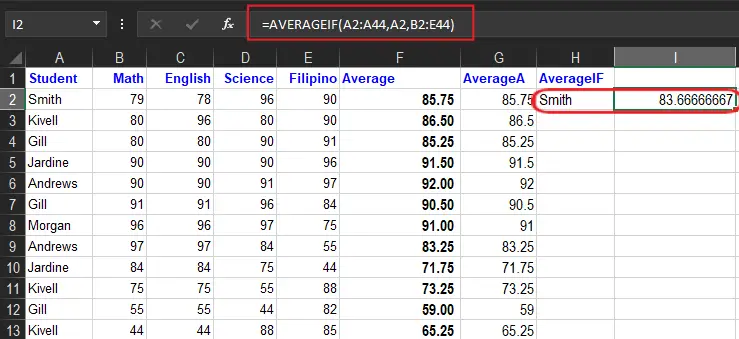
- Select the cell I3.

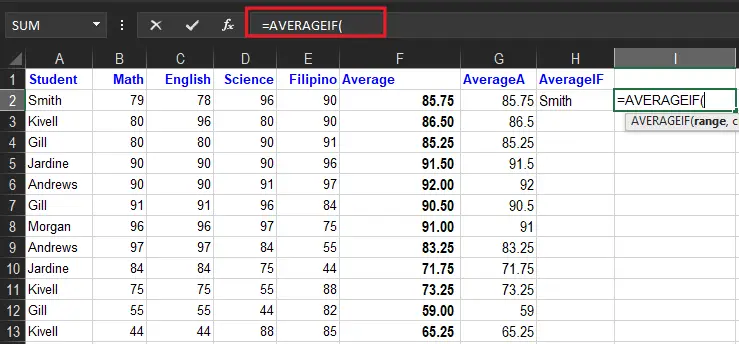
- Type =AVERAGEIF.

- Double-click the AVERAGEIF command.
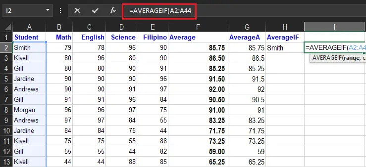
- Specify the range for the condition
A2:A44. Ranges of students’ names.
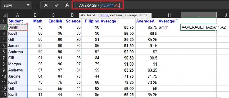
- Type comma(
,)
- Specify the criteria (the cell A2, which has the value “Smith”)

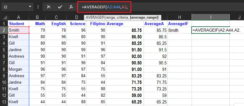
- Type comma(
,)
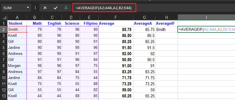
- Specify the range for the average
B2:E44.
- Press Enter to see the result.

How to use AVERAGEIF Function in Excel
Microsoft Excel has provided a built-in function that can be used in a spreadsheet. So here, we’ll now look at how to utilize the following examples and steps provided.
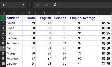
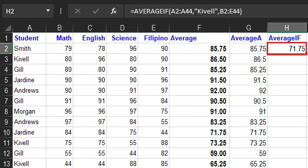
As AVERAGEIF discussed above, the main idea of it is to find the average of the cells in an exact match of criterion. For instance, here we wish to find the average of students’ grades.
Example 1:
We provide here the given sample data:
The formula used to find the average is below:
Wildcards
Now in creating criteria in AverageIf function Excel you can use the wildcards characters. Namely, characters question mark (?), asterisks(*), or tilde (~). Additionally, the question mark(?) matches one character and the asterisk matches zero or more characters of any kind.
For example, to average cells in a B1:B10 when cells in A1:A10 contain the text “Smith” anywhere, you can use a formula like this:
=AVERAGEIF(A1:A10,"*Smith*",B1:B10)
Things to remember about the AVERAGEIF Function
- The AVERAGEIF treats 0 as value if the given criteria is empty.
- #DIV0! error-Occurs when:
- No cells that meet the range of the criteria.
- Range is empty or string value.
- The function will ignore cells that contain TRUE or FALSE.
- The use of wildcard characters such as the asterisk (*), the tilde(~) in the function as criteria, greatly enhances the search criteria.
Summary
In summary, we discussed and learn the AVERAGEIF Function with the following concept:
- Average_range does not have to be the same size as range. The top left cell in average_range is used as the starting point, and cells that correspond to cells in range are averaged.
- Cells in range that contain TRUE or FALSE are ignored.
- Empty cells are ignored in range and average_range when calculating averages.
- AVERAGEIF returns #DIV/0! if no cells in range meet criteria.
- AVERAGEIF allows the wildcard characters question mark (?) and asterisk (*), in criteria. The question mark ? matches any single character and the asterisk(*) matches any sequence of characters. To find a literal (?) or *, use a tilde (~) before the character, i.e. ~* and ~?.

Glay Eliver
Programmer & Technical Writer at PIES IT Solution
Glay Eliver is a programmer and writer at PIES IT Solution, author of over 600 tutorials at itsourcecode.com. Specializes in JavaScript tutorials, Microsoft Office how-tos (Excel, Word, PowerPoint), and Python error debugging covering ImportError, TypeError, AttributeError, ModuleNotFoundError, and JavaScript ReferenceError. Authored several of the site’s highest-traffic Excel and MS Office reference articles.
Expertise: JavaScript · MS Excel · MS Word · MS PowerPoint · Python · Python ImportError · Python TypeError · Python AttributeError · ModuleNotFoundError · JavaScript ReferenceError · Pygame · View all posts by Glay Eliver →