
This time we will briefly discuss the Excel filter function with examples along with basic formulas that you can understand quickly.
What formula or tool are you using in filtering? Are you using Autofilter or advanced way of filtering? However, these methods have drawbacks which do not update automatically when data changes.
The introduction of the FILTER function in Excel 365 becomes a long-awaited alternative to conventional features. Unlike them, Excel formulas recalculate automatically with each worksheet change, so you’ll need to set up your filter just once!
What is excel filter function?
The filter function is used to return range of filtered data based on the criteria you define. This function can handle multiple criteria and belong to the dynamic arrays function category.
The output of this function is an array of values that automatically spills into a range of cells, starting from the cell where you enter a formula.
On working this function here is the syntax you may use:
FILTER(array, include, [if_empty])
Where the arguments are as follows:
- Array – It is required and its the range or array of values that you want to filter.
- Include – It is a required argument thus the boolean array criteria are supplied. (TRUE or FALSE value).
- If_empty argument is optional and this is the value to return when the input data does meet the criteria.
Reminder: Unfortunately, this function is not available on the earlier versions such MS Excel 2019, Excel 2016 thus it is only present on Microsoft 365 and Excel 2021 and online spreadsheet.
Basic filter function excel
To begin let’s focus on the basic filtering formula of excel, which is going to be a simple scenario for clarification and easy understanding.
For instance to pull values from A2:A20 with less than 75 the formula is shown below:
=FILTER(A2:A20,A2:A20<75)To get the value of A2:E20 wherein the A2:A20 is greater than 75 the formula is shown below:
=FILTER(A2:E20,A2:A20>75)As you observe the second formula range of arrays and the logic is the same.
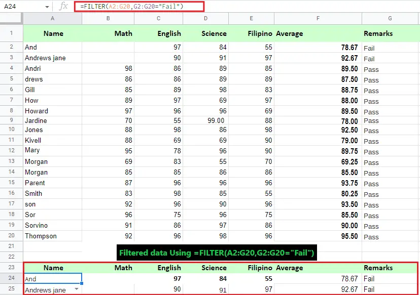
Apparently, we are going to student lists of grades, so that we will know who failed. In our example below, we filtered the cells A2:G20 by their remarks: Fail. As you can see it creates a table containing Failed students.
=FILTER(A2:G20,G2:G20="Fail")
How to use filter function in excel
Currently that you know how to do basic filter function and formulas, it’s time to work on a bit more complex but can contribute more understanding and skills in excel.
Excel filter function multiple criteria
So the excel filter function with multiple criteria requires two or more logical expressions on the include argument. The syntax of this formula is given below.
=FILTER(array, (range1=criteria1) * (range2=criteria2), "No results")
Technically this formula works well with help of multiplication operations and AND logic which processes the arrays and ensures that all the criteria meet and are returned,
To elaborate the logical expression is the array values of Boolean, which if there’s a value of 1 is TRUE and 0 equates False. Then all the elements of an array are multiplied within the same position.
Since when we multiply zero by zero it always yields zero then only the items for which all the criteria are TRUE get into the resulting array, and consequently only those items are extracted.
For example, to extract only data where the group is “math” and grades is less than 75, wherein the math and grades are the same column range you can use a formula like this:
=FILTER(range,(subject="math")*(grades<75),"No results")Excel filter function multiple columns
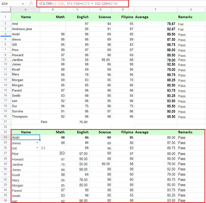
It’s time to filter multiple columns in excel as we know how to filter multiple criteria. In our case we will filter two columns average and remarks.
With these columns we set the criteria needed to extract the correct filter, the first criteria average which is greater than or equal to 75, and the remarks which is Pass
Afterward, the array range of data A2:G20 will be the source of the next range F2:F20 and G2:G20 which we can up the following formula:0
=FILTER(A2:G20, (F2:F20>=C21) * (G2:G20=B21), "No results")As the result, you get a list of students who passed and grades greater than 75.
Filter Excel Shortcut
The keyboard filter Excel short is to Press CTRL+SHIFT+L. Additionally, this shortcut is to filter the active cell data in Excel however if you want to remove it just press again the short cut key. For instance, if you want to open the filter dialog box press CTRL+SHIFT+F.
Excel Advanced Filter
Excel advanced filter is an advance version of excel filtering but it’s an underrated feature of excel. Thus this is helpful when you want to filter multiple criteria in your data set.
For instance, if you want to extract a unique list it’s fascinating to use especially if you want to get rid of duplicates entry.
Here are the steps to get all the unique records:
- Select all the data you want to filter including headers.
- On the Data tab>Sort & Filter> Advanced. Instead, you can use Alt + A + Q. Then the advanced filter dialog box will open.
- In the Advanced Filter dialog box, you will see the following:
- Action: Select the ‘Copy to another location’ option. This will give you where you want to get the unique records.
- List Range: Your data set must be referring to the unique records you want to get. Also, make sure headers in the data set are included.
- Criteria Range: Make this empty.
- Copy To: Specify the cell address where you want to get the list of unique records.
- Copy Unique Records Only: Check this option.
- Click OK.
Caution: If using Advanced Filter to extract a unique list keep in mind to also select the header otherwise the first cell will be determined as the header.
Conclusion
To sum up we have learned Excel Filter Function With Examples and Basic Formulas. Hence this formula is easy to work and use when you are trying to filter your data. Additionally, we came up with the following conclusion:
- FILTER can perform with both horizontal and vertical arrays.
- The FILTER will return #VALUE! if include argument location is not compatible with array argument.
- Thus FILTER will return error if the inlude_array contains an error.
See you on our next tutorial!

Glay Eliver
Programmer & Technical Writer at PIES IT Solution
Glay Eliver is a programmer and writer at PIES IT Solution, author of over 600 tutorials at itsourcecode.com. Specializes in JavaScript tutorials, Microsoft Office how-tos (Excel, Word, PowerPoint), and Python error debugging covering ImportError, TypeError, AttributeError, ModuleNotFoundError, and JavaScript ReferenceError. Authored several of the site’s highest-traffic Excel and MS Office reference articles.
Expertise: JavaScript · MS Excel · MS Word · MS PowerPoint · Python · Python ImportError · Python TypeError · Python AttributeError · ModuleNotFoundError · JavaScript ReferenceError · Pygame · View all posts by Glay Eliver →