How to Freeze Rows in Google Sheets (2026)

Freezing rows or columns in Google Sheets keeps them visible while you scroll through large datasets. Header rows stay locked at the top, and reference columns stay pinned on the left. This 2026 guide covers freezing single rows, multiple rows, columns, unfreezing, mobile app, and best practices.

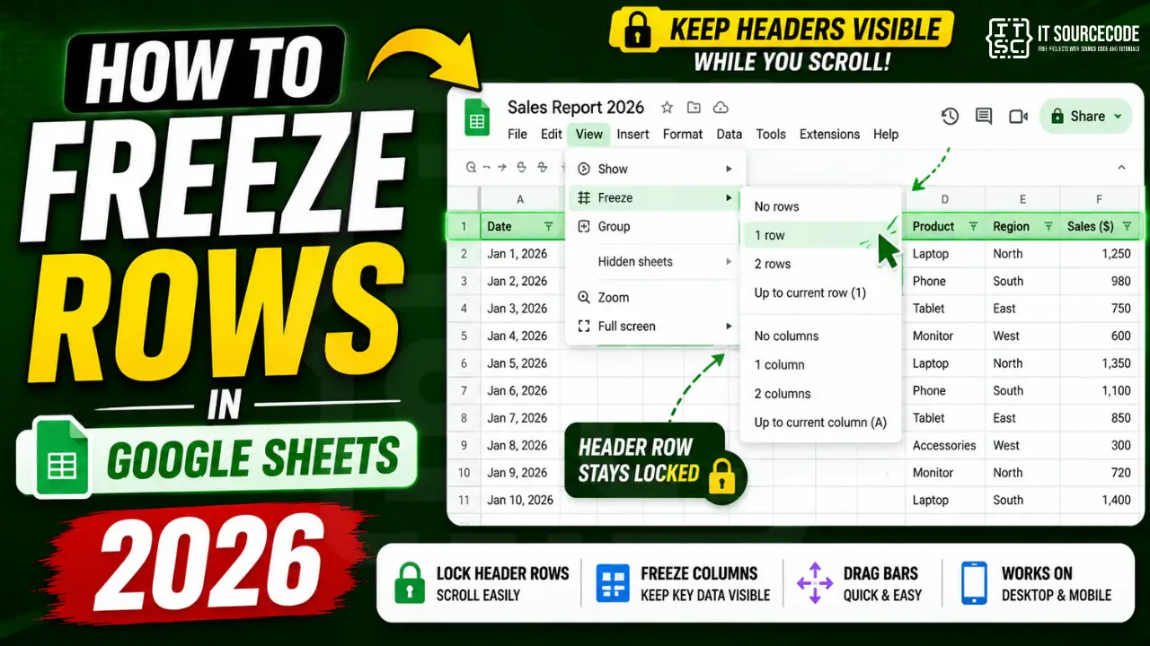
How to freeze the first row (header)

1. Open your Google Sheets file.
2. Click View in the top menu.
3. Hover over Freeze.
4. Click 1 row.
5. Row 1 stays locked as you scroll down.

How to freeze multiple rows

1. Click the row number below the last row you want to freeze (e.g., click row 4 to freeze rows 1-3).
2. Go to View > Freeze > Up to current row (3).
3. Or: View > Freeze > 2 rows for exactly 2 rows.

Available freeze options for rows:
- No rows
- 1 row
- 2 rows
- Up to current row (N)

How to freeze columns

1. Click the column letter to the right of the last column you want to freeze.
2. Go to View > Freeze > Up to current column.
3. Or: View > Freeze > 1 column or 2 columns.

Frozen columns stay visible as you scroll right through wide sheets.

Freeze both rows AND columns

You can combine row and column freezes:

1. Click cell B2.
2. View > Freeze > 1 row (freezes row 1).
3. View > Freeze > 1 column (freezes column A).
4. Now row 1 and column A both stay pinned while you scroll anywhere.

Freeze using drag handles (mouse method)

Google Sheets shows gray horizontal and vertical bars at the top-left of the grid:

• Horizontal freeze bar: on top of row 1, between the column header letters and the data. Drag it down to freeze rows above it.
• Vertical freeze bar: on the left of column A, between the row numbers and the data. Drag it right to freeze columns left of it.

Quick visual method for freezing exactly the rows/columns you want.

How to unfreeze rows and columns

1. Go to View > Freeze.
2. Click No rows to unfreeze rows.
3. Click No columns to unfreeze columns.

Or drag the freeze bars back to their original position (top-left corner of the grid).

Freezing on Google Sheets mobile app (iPhone / Android)

1. Open the sheet in the Google Sheets app.
2. Tap and hold the row number (or column letter).
3. Tap the three-dot menu that appears.
4. Tap Freeze.

Alternate method: tap-and-hold the row number, then drag it slightly. A freeze option appears in the toolbar.

Best practices for freezing

• Always freeze row 1 on data tables with headers, so users see column names as they scroll.
• Freeze up to 3 rows if you have report titles above headers.
• Freeze the first column when it contains identifiers (customer name, product code).
• Do NOT freeze too many rows or columns; you lose viewing space.
• Combine freeze with pane split for complex dashboards (Format > Alternating colors reinforces frozen headers visually).

Freeze vs Hide vs Group rows

• Freeze: keeps rows/columns visible while scrolling. Great for headers.
• Hide: removes rows/columns from view entirely. Great for hiding calculation rows.
• Group: allows collapsing/expanding rows. Great for outlined reports.

Common freeze issues

• Freeze not visible: the horizontal separator line indicates the freeze boundary. If missing, freeze may not be applied, retry via View menu.
• Frozen rows visible but scrolling awkward: too many rows frozen. Reduce to 1-3 rows max.
• Frozen area disappears when sharing: recipient’s view may load without freeze. They can enable it via View > Freeze on their end.
• Cannot freeze on mobile: some older Android versions had bugs. Update Sheets app.