How to Use SUMIF in Google Sheets (2026)

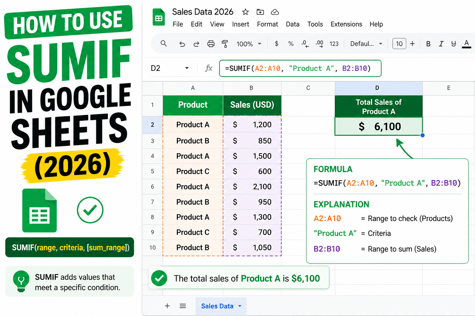
SUMIF adds up numbers that match a single condition. SUMIFS handles multiple conditions at once. Both are essential for financial reports, sales summaries, inventory totals, and any analysis where you sum specific rows in a table. Here is the complete 2026 guide to SUMIF and SUMIFS in Google Sheets with 15 practical examples.

SUMIF syntax

=SUMIF(range, criterion, [sum_range])

• range: the cells to test against the criterion.
• criterion: the condition (like “>100” or “Ana” or “<=0”).
• sum_range: optional. The cells to sum if the corresponding range cell meets criterion. If omitted, sums the range itself.

Basic SUMIF examples

Sum all values in B2:B10 greater than 100:
=SUMIF(B2:B10, ">100")

Sum all sales for customer "Ana":
=SUMIF(A2:A10, "Ana", B2:B10)

Sum sales for products starting with "PROD":
=SUMIF(A2:A10, "PROD*", B2:B10)

Sum sales for exactly 500 (equal to):
=SUMIF(B2:B10, 500)

Sum negative values only:
=SUMIF(B2:B10, "<0")

SUMIFS syntax (multiple conditions)

=SUMIFS(sum_range, criteria_range1, criterion1, [criteria_range2, criterion2, ...])

Note: SUMIFS has sum_range FIRST (unlike SUMIF which has it last). Each additional criteria comes as a pair (range + criterion).

SUMIFS examples

Sum sales for Ana in Q2:
=SUMIFS(C:C, A:A, "Ana", B:B, "Q2")

Sum sales over 100 for VIP customers:
=SUMIFS(C:C, D:D, "VIP", C:C, ">100")

Sum for date range (all of 2026):
=SUMIFS(C:C, B:B, ">=1/1/2026", B:B, "<=12/31/2026")

Sum sales where region=West AND product=A:
=SUMIFS(C:C, A:A, "West", B:B, "A")

Sum quantity for orders that shipped:
=SUMIFS(B:B, C:C, "Shipped")

Using cell references in criteria (dynamic)

Instead of hardcoding criteria, use cell references so users can change values:

Cell F1 contains: Ana

Formula:
=SUMIF(A2:A10, F1, B2:B10)

Or with condition operators:
Cell F1 contains: 100
=SUMIF(B2:B10, ">"&F1)

The ampersand (&) concatenates the operator with the cell value.

Wildcards in SUMIF

Sum for anything starting with "PROD":
=SUMIF(A2:A10, "PROD*", B2:B10)

Sum for anything ending with "-A":
=SUMIF(A2:A10, "*-A", B2:B10)

Sum for anything containing "phone":
=SUMIF(A2:A10, "*phone*", B2:B10)

Sum for exact 3-character codes:
=SUMIF(A2:A10, "???", B2:B10)

SUMIF with dates

Sum sales after Jan 1, 2026:
=SUMIF(A2:A10, ">="&DATE(2026,1,1), B2:B10)

Sum sales in a specific month:
=SUMIFS(C2:C10, A2:A10, ">="&DATE(2026,7,1), A2:A10, "<="&DATE(2026,7,31))

Sum sales in current month:
=SUMIFS(C:C, A:A, ">="&EOMONTH(TODAY(),-1)+1, A:A, "<="&EOMONTH(TODAY(),0))

Common SUMIF and SUMIFS errors

• #REF! error: range and sum_range are different sizes. They must have the same number of rows.
• #VALUE! error: criterion contains an invalid comparison. Check operators and quotes.
• Returns 0: no rows match criteria. Verify data types (text vs number, dates formatted correctly).
• SUMIFS syntax confusion: sum_range is FIRST, not last. This is opposite of SUMIF.
• Text vs number mismatch: “100” as text does not match 100 as number. Ensure consistency.

Real-world SUMIF use cases

• Monthly sales summary by rep: SUMIFS to break down sales by rep + month.
• Expense report by category: SUMIF to total each category (food, transport, utilities).
• Inventory count by supplier: SUMIF to count units by supplier ID.
• Grade class average conditional: SUMIF to average only passing scores.
• Budget tracking: SUMIFS to sum spent amount within date range and category.

Advanced SUMIF patterns for real work

Basic SUMIF works well for single-condition sums, but real spreadsheets need more. Here are the three advanced patterns I use most often in 2026 for business and capstone data analysis.

SUMIFS for multiple conditions

SUMIFS extends SUMIF with additional criteria. Example: sum sales where product is “Laptop” AND region is “NCR”: =SUMIFS(sales_range, product_range, "Laptop", region_range, "NCR"). Order matters: sum range comes first in SUMIFS, unlike SUMIF where it comes last.

SUMIF with wildcards for partial match

Use * to match any string and ? to match one character. Example: sum sales for all products starting with “Lap”: =SUMIF(product_range, "Lap*", sales_range). Great for grouping similar categories without exact-match cleanup work.

SUMIF with comparison operators

Use operators inside the criteria string. Sum sales greater than 10,000: =SUMIF(sales_range, ">10000"). Sum sales for dates after Jan 1: =SUMIF(date_range, ">=" & DATE(2026,1,1), sales_range). This lets you build dynamic threshold reports without writing IF statements.

Common SUMIF mistakes to avoid

SUMIF looks simple but has quirks that cause subtle bugs. Here are the five mistakes I see most often and how to fix each one.

• Range mismatch between criteria and sum ranges. If criteria range is A2:A100 but sum range is B2:B50, SUMIF only sums the first 49 matches then breaks. Make both ranges the same size.
• Text criteria without quotes. =SUMIF(A2:A100, Laptop, B2:B100) fails because Laptop is treated as a cell reference. Wrap text in quotes: "Laptop".
• Case sensitivity confusion. SUMIF is not case-sensitive. It treats “Laptop” and “LAPTOP” as the same match. If you need case-sensitive matching, use SUMPRODUCT with EXACT.
• Wildcards do not work on numbers. =SUMIF(A2:A100, "1*", B2:B100) does not match numbers starting with 1. Convert numbers to text first or use SUMIFS with comparison operators.
• Whitespace in criteria data. “Laptop” with a trailing space does not match “Laptop” without one. Use TRIM to clean data before sum: =SUMPRODUCT((TRIM(A2:A100)="Laptop") * B2:B100).

For most business dashboards in 2026, SUMIFS covers 90 percent of your aggregation needs. Reach for SUMPRODUCT only when you need complex logic like AND across text conditions with wildcards. Keep formulas simple and add helper columns when the logic gets nested.

For any spreadsheet you plan to share with teammates or a client, add a comment cell explaining what each SUMIF formula does. Complex conditional logic is unreadable at a glance six months later even to the person who wrote it. Two lines of explanation save hours of confused debugging.

Adrian Mercurio

Full-Stack Developer at PIES IT Solution

Adrian Mercurio is a full-stack developer at PIES IT Solution. Specializes in building complete capstone projects with full documentation. Strong background in PHP/MySQL development and database design. Has personally built and tested over 30 capstone-ready projects with ER diagrams, DFDs, and chapter-by-chapter thesis documentation.

Expertise: PHP, Laravel, Database Design, Capstone Projects, C#, C, C++, Python, AI Projects  · View all posts by Adrian Mercurio →