How to Use IF Function in Google Sheets (2026)

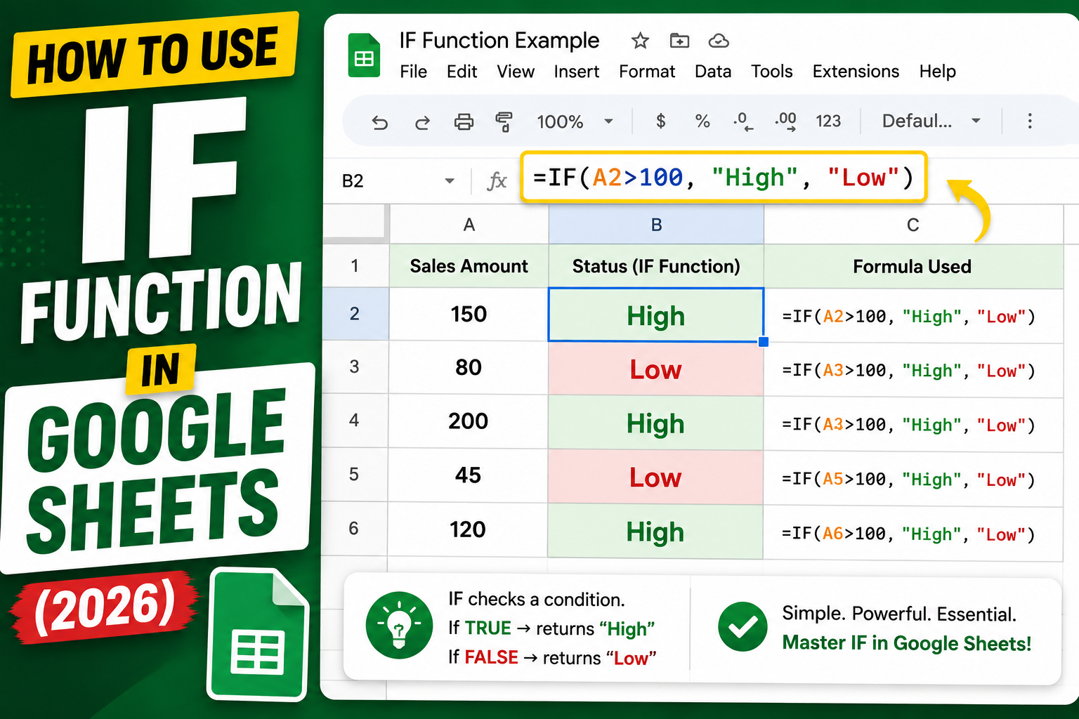
The IF function in Google Sheets is the most versatile logical function. It tests a condition and returns different values based on whether the condition is TRUE or FALSE. Simple to learn, powerful in combination with other functions. Here is the complete 2026 guide to IF in Google Sheets, including nested IF, IFS function, and IF combined with AND, OR, VLOOKUP, and SUM.

IF function syntax

=IF(logical_expression, value_if_true, value_if_false)

• logical_expression: any comparison that returns TRUE or FALSE (like A1>100).
• value_if_true: what to return if the condition is TRUE.
• value_if_false: what to return if the condition is FALSE (optional in some contexts).

Basic IF examples

Pass or Fail based on grade:
=IF(A2>=75, "Pass", "Fail")

Bonus based on sales:
=IF(B2>100000, "Bonus Earned", "No Bonus")

Discount flag for VIP customers:
=IF(C2="VIP", "10% off", "No discount")

Empty vs filled cell:
=IF(A2="", "Empty", "Filled")

Categorize spending:
=IF(D2<=100, "Low", "High")

Common comparison operators

• = equal to
• <> not equal to
• > greater than
• < less than
• >= greater than or equal to
• <= less than or equal to

Nested IF for multiple conditions

To check multiple conditions in order, put an IF inside another IF:

Grade letter from score:
=IF(A2>=90, "A", IF(A2>=80, "B", IF(A2>=70, "C", IF(A2>=60, "D", "F"))))

Read left to right: if score is 90+, return A. Otherwise if 80+, return B. And so on. The last IF returns F for anything below 60.

IFS function: cleaner alternative to nested IF

Google Sheets has an IFS function that handles multiple conditions without nesting:

=IFS(A2>=90, "A",
     A2>=80, "B",
     A2>=70, "C",
     A2>=60, "D",
     TRUE, "F")

Each pair is a condition followed by its return value. TRUE at the end acts as a catch-all default (like “else” in programming).

IF combined with AND or OR

Check multiple conditions simultaneously:

Pass only if score>=75 AND attendance>=80%:
=IF(AND(A2>=75, B2>=0.8), "Pass", "Fail")

Discount if customer is VIP OR has spent over 10,000:
=IF(OR(C2="VIP", D2>=10000), "10% off", "No discount")

Complex example with both:
=IF(AND(A2>=90, OR(B2="Gold", C2="Platinum")), "Top Tier", "Standard")

IF combined with VLOOKUP

Return message if VLOOKUP finds product, else show "Not stocked":
=IF(IFERROR(VLOOKUP(A2, Products!A:A, 1, FALSE), FALSE), "In stock", "Not stocked")

SUMIF and COUNTIF (IF-based sum and count)

Sum all sales over 1000:
=SUMIF(B:B, ">1000")

Count all VIPs:
=COUNTIF(C:C, "VIP")

Count non-empty cells:
=COUNTIF(A:A, "<>")

Sum sales for customer "Ana":
=SUMIF(A:A, "Ana", B:B)

IF for error handling with IFERROR

Wrap risky formulas in IFERROR to show a message instead of #DIV/0!, #N/A, or #REF!:

Show "-" if division by zero:
=IFERROR(A2/B2, "-")

Show blank if VLOOKUP fails:
=IFERROR(VLOOKUP(D2, Products!A:B, 2, FALSE), "")

Common IF function mistakes

• Forgetting quotes around text: =IF(A2=Pass, ...) fails. Should be =IF(A2="Pass", ...)
• Wrong operator: use = for equality (not ==).
• Too many nested IFs: hard to read past 4 levels. Use IFS instead.
• Comparing text with numbers: =IF(A2="100", ...) may fail if A2 contains the number 100 (not text). Use =IF(A2=100, ...) for numbers.
• Missing FALSE branch: some contexts require both TRUE and FALSE branches. Add a blank string “” if you have nothing to return.

Advanced IF patterns: IFS, nested IF, and combining with AND/OR

Once you know the basic IF syntax, three advanced patterns solve most real-world logic problems in Google Sheets. Here is when to use each.

Use IFS for multiple conditions in sequence

When you need to check 3 or more conditions in order, use IFS instead of nesting IF statements. It reads left to right and returns the first matching result. Example: =IFS(A2>90, "A", A2>80, "B", A2>70, "C", TRUE, "F"). The TRUE at the end catches everything that did not match earlier conditions.

Combine IF with AND/OR for compound logic

When you need multiple conditions to be true at the same time, wrap them with AND. Example: =IF(AND(A2>0, B2>0), "Both positive", "One or both invalid"). Use OR when any single condition can trigger the result. Example: =IF(OR(A2="new", A2="pending"), "Needs review", "Done").

Nested IF for tiered decisions

Sometimes you need one IF result to depend on another. Nesting IFs works but gets hard to read past 3 levels. Example: =IF(A2>100, IF(B2="urgent", "priority", "normal"), "skip"). When your nested IF is more than 3 levels deep, refactor with IFS or restructure your data. Nested IF at 5 levels is unmaintainable.

Common IF function mistakes to avoid

Even experienced spreadsheet users make these IF mistakes. Fix them and your formulas will be more reliable and easier to debug.

• Missing quotation marks around text. =IF(A2="pass", "Good", "Retry") works but =IF(A2=pass, "Good", "Retry") does not. Text values inside IF conditions must be wrapped in double quotes.
• Confusing comma with semicolon. If you are using Google Sheets in a European locale, arguments may be separated by semicolons instead of commas. Match your locale settings.
• Using = for exact match on numbers with decimals. Floating-point math means 0.1+0.2 is not exactly 0.3. Use ROUND or <= comparisons when checking decimal equality.
• Nesting too deep. If your IF has more than 3 levels of nesting, refactor with IFS, SWITCH, or a lookup table. Deep nesting is unreadable and error-prone.
• Not accounting for empty cells. =IF(A2>0, "yes", "no") returns “no” for empty cells, which may not be what you want. Use =IF(ISBLANK(A2), "", IF(A2>0, "yes", "no")) to skip empty cells cleanly.

My tip for anyone building spreadsheet logic in 2026: prefer IFS over deeply nested IF, and use named ranges to make your formulas more readable. Complex IF logic that someone else has to maintain is a maintenance burden. Simpler is better even when it means an extra column.

Adrian Mercurio

Full-Stack Developer at PIES IT Solution

Adrian Mercurio is a full-stack developer at PIES IT Solution. Specializes in building complete capstone projects with full documentation. Strong background in PHP/MySQL development and database design. Has personally built and tested over 30 capstone-ready projects with ER diagrams, DFDs, and chapter-by-chapter thesis documentation.

Expertise: PHP, Laravel, Database Design, Capstone Projects, C#, C, C++, Python, AI Projects  · View all posts by Adrian Mercurio →