How to Use VLOOKUP in Google Sheets (2026)

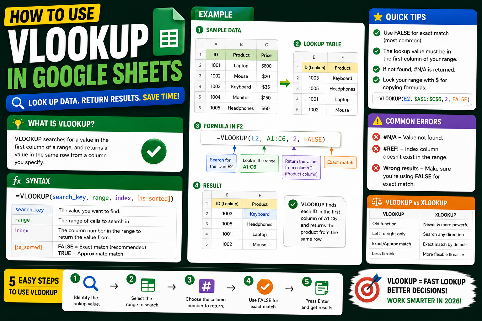
VLOOKUP is the most popular Google Sheets lookup function. It finds a value in the first column of a range and returns a value from another column in the same row. Used for price lists, customer databases, employee records, and any table where you need to pull related data. Here is the complete 2026 guide to VLOOKUP in Google Sheets with syntax, examples, error handling, and when to use INDEX MATCH instead.

VLOOKUP syntax

=VLOOKUP(search_key, range, index, [is_sorted])

• search_key: the value you are looking for (like a customer ID or product code).
• range: the table where the search happens. First column must contain search_key values.
• index: column number to return. 1 = first column of range, 2 = second column, etc.
• is_sorted: TRUE for approximate match (data must be sorted). FALSE for exact match. Almost always use FALSE.

Basic VLOOKUP example: Get price from product code

Suppose you have this product list in cells A2:B10:

A       B
PROD01  150.00
PROD02  225.50
PROD03  89.99
PROD04  340.00

Formula to look up PROD02’s price:

=VLOOKUP("PROD02", A2:B10, 2, FALSE)
Result: 225.50

VLOOKUP with cell reference (dynamic)

Instead of typing the search key, reference a cell so the formula is reusable:

Cell D2 contains: PROD02

Formula in E2:
=VLOOKUP(D2, A2:B10, 2, FALSE)
Result: 225.50

Change D2 to any product code and E2 updates automatically.

VLOOKUP across different sheets

Reference another sheet using the sheet name + exclamation mark:

=VLOOKUP(A2, 'Products'!A:C, 3, FALSE)

Looks up A2 value in the ‘Products’ sheet, returns the 3rd column. Wrap sheet name in single quotes if it contains spaces or special characters.

VLOOKUP across different Google Sheets files

Use IMPORTRANGE combined with VLOOKUP to pull data from another workbook:

=VLOOKUP(A2, IMPORTRANGE("spreadsheet_URL", "Sheet1!A:C"), 3, FALSE)

Note: you must click “Allow access” the first time you use IMPORTRANGE with a new spreadsheet URL.

Handle #N/A errors with IFERROR

VLOOKUP returns #N/A when the search key is not found. Wrap in IFERROR to show a friendlier message:

=IFERROR(VLOOKUP(D2, A2:B10, 2, FALSE), "Not found")

Alternative: return 0 instead:
=IFERROR(VLOOKUP(D2, A2:B10, 2, FALSE), 0)

Common VLOOKUP errors and fixes

• #N/A error: search key not found. Check spelling, spaces before/after values, and column formatting (text vs number).
• #REF! error: index number exceeds the number of columns in range. If range has 3 columns, index must be 1, 2, or 3.
• #VALUE! error: index is 0 or negative. Index must be 1 or greater.
• Returns wrong value: you likely have is_sorted set to TRUE with unsorted data. Change to FALSE for exact match.
• Case-sensitivity: VLOOKUP is NOT case-sensitive. “PROD02” and “prod02” both match. For case-sensitive lookup, use INDEX MATCH with EXACT.

VLOOKUP limitations

• Can only look up left-to-right: search column must be leftmost. Cannot return values from columns to the left of the search column.
• Index number is fragile: adding or deleting columns breaks VLOOKUP. INDEX MATCH is more robust.
• Not case-sensitive: for case-sensitive lookups use INDEX MATCH + EXACT.
• Slow on large datasets: for tables over 100,000 rows, use FILTER or QUERY instead.

VLOOKUP vs INDEX MATCH: which to use

• Use VLOOKUP when the search column is leftmost and you need a quick simple lookup.
• Use INDEX MATCH when you need to look up left of the search column, OR when the source data structure may change, OR when you need case-sensitive lookup.
• INDEX MATCH is slightly more complex but more powerful. Many Sheets power users use INDEX MATCH exclusively.

Real-world VLOOKUP examples

Employee salary lookup:

=VLOOKUP(A2, 'Employees'!A:D, 4, FALSE)
Looks up employee ID from A2 in Employees sheet, returns column 4 (salary).

Customer information lookup:

=VLOOKUP(A2, 'Customers'!A:F, 6, FALSE)
Returns customer email based on customer ID.

Grade letter from score:

Grade table sorted ascending:
A2: 0    B2: F
A3: 60   B3: D
A4: 70   B4: C
A5: 80   B5: B
A6: 90   B6: A

Formula (TRUE for approximate match):
=VLOOKUP(85, A2:B6, 2, TRUE)
Result: B

Common VLOOKUP mistakes to avoid

Even experienced Google Sheets users hit VLOOKUP errors. Most of them come from the same handful of mistakes. Here are the six patterns I see most often, and how to fix each one.

• Lookup value is in a column to the right of your return column. VLOOKUP only searches left to right. If you want to look up a value in column C and return a value from column A, VLOOKUP will not work. Use INDEX MATCH or XLOOKUP instead, or restructure your data.
• Forgetting the fourth argument (FALSE for exact match). When you leave the fourth argument blank or set it to TRUE, VLOOKUP does approximate matching, which returns wrong values for unsorted data. Always add FALSE as the fourth argument unless you specifically need approximate match.
• Mixing text and number data types. If your lookup value is the number 123 but your source column contains the text “123” (or vice versa), VLOOKUP returns #N/A. Use =VALUE() or =TEXT() to convert data types so both sides match.
• Extra spaces in your data. “Product A” and “Product A ” (with a trailing space) look identical but VLOOKUP treats them as different. Wrap your lookup value with =TRIM() to strip whitespace before comparison.
• Not locking your range with dollar signs. When you drag the VLOOKUP formula down, the range shifts too. Use absolute references like $A$2:$D$100 so the range stays fixed while the lookup value moves.
• Using column letters instead of column numbers in the third argument. The third argument is the column index (a number), not the letter. If you type D instead of 4, Google Sheets throws an error.

VLOOKUP vs XLOOKUP: which one to use in 2026

Google Sheets rolled out XLOOKUP in 2022, and it has become the recommended lookup function for most new spreadsheets. VLOOKUP still works, but XLOOKUP fixes the biggest limitations. Here is how to decide which to use.

Use XLOOKUP when…

You need to look up a value in any direction (left, right, up, or down). XLOOKUP does not require your lookup column to be first. It also handles #N/A errors natively with a built-in default value, so you can skip the IFERROR wrapper: =XLOOKUP("Product A", A2:A100, D2:D100, "Not found").

Use VLOOKUP when…

You are collaborating with a team on older spreadsheets, or you are working with clients who have not adopted XLOOKUP yet. VLOOKUP has been in Google Sheets since day one, so every user recognizes it. XLOOKUP is newer and some macros or scripts do not support it yet.

Quick syntax comparison

// VLOOKUP: 4 arguments, only searches right
=VLOOKUP(lookup_value, range, column_index, [is_sorted])
=VLOOKUP("Product A", A2:D100, 4, FALSE)

// XLOOKUP: cleaner syntax, searches any direction
=XLOOKUP(lookup_value, lookup_range, return_range, [if_not_found])
=XLOOKUP("Product A", A2:A100, D2:D100, "Not found")

// INDEX MATCH: the classic pre-XLOOKUP workaround
=INDEX(D2:D100, MATCH("Product A", A2:A100, 0))

My rule of thumb: use XLOOKUP for all new formulas you write in 2026 and beyond. Keep VLOOKUP alive on existing formulas until you are ready to refactor. Do not mix both in the same spreadsheet without a good reason, or your teammates will get confused when they inherit the file.

Adrian Mercurio

Full-Stack Developer at PIES IT Solution

Adrian Mercurio is a full-stack developer at PIES IT Solution. Specializes in building complete capstone projects with full documentation. Strong background in PHP/MySQL development and database design. Has personally built and tested over 30 capstone-ready projects with ER diagrams, DFDs, and chapter-by-chapter thesis documentation.

Expertise: PHP, Laravel, Database Design, Capstone Projects, C#, C, C++, Python, AI Projects  · View all posts by Adrian Mercurio →