How to Use ARRAYFORMULA in Google Sheets (2026)

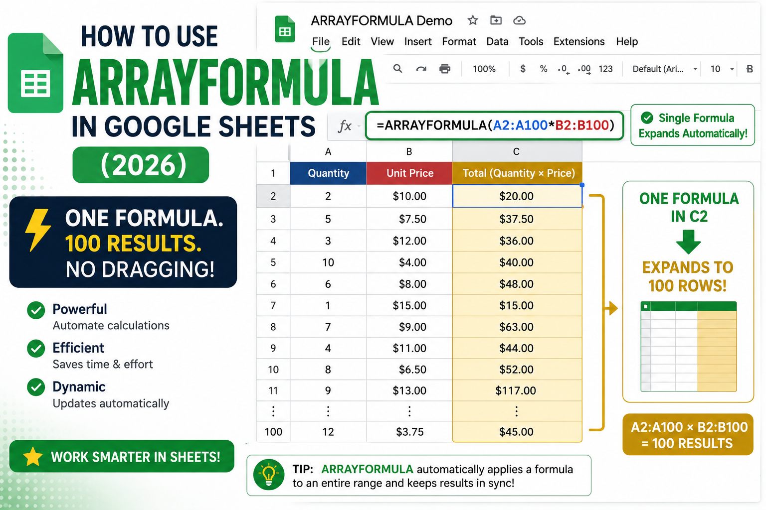
ARRAYFORMULA is a Google Sheets exclusive that applies one formula to an entire range or column at once. Instead of dragging a formula down 1,000 rows, one ARRAYFORMULA fills them all automatically. It also updates itself when new rows are added. This 2026 tutorial shows every essential ARRAYFORMULA pattern with real examples.

ARRAYFORMULA syntax

=ARRAYFORMULA(array_formula)

Short form: press Ctrl+Shift+Enter after typing formula
(Sheets auto-wraps with ARRAYFORMULA)

Basic ARRAYFORMULA examples

Multiply two columns row-by-row (in cell C2, fills C2:C1000):
=ARRAYFORMULA(A2:A1000 * B2:B1000)

Add two columns:
=ARRAYFORMULA(A2:A + B2:B)

Concatenate first + last name:
=ARRAYFORMULA(A2:A & " " & B2:B)

Calculate percentage of total:
=ARRAYFORMULA(B2:B / SUM(B2:B) * 100)

Round all values in a range:
=ARRAYFORMULA(ROUND(B2:B, 2))

Note: A2:A means “column A from row 2 to end of column”, an open-ended range that grows as data is added.

ARRAYFORMULA with IF

Grade all students in column B:
=ARRAYFORMULA(IF(B2:B>=75, "Pass", "Fail"))

Skip blank rows:
=ARRAYFORMULA(IF(B2:B="", "", IF(B2:B>=75, "Pass", "Fail")))

Nested IF for grade letters:
=ARRAYFORMULA(IF(B2:B="", "",
  IF(B2:B>=90, "A",
   IF(B2:B>=80, "B",
    IF(B2:B>=70, "C", "F")))))

ARRAYFORMULA with VLOOKUP

Look up prices for all product codes at once:
=ARRAYFORMULA(IF(A2:A="", "", VLOOKUP(A2:A, Products!A:C, 3, FALSE)))

- Skips blanks with IF wrapper.
- Applies VLOOKUP to each row of A2:A.

ARRAYFORMULA with SUMIF (running total)

Running total per customer:
=ARRAYFORMULA(IF(A2:A="", "", SUMIF(A2:A, A2:A, B2:B)))

- Sums B for each unique value in A.
- Great for customer totals, category sums.

Auto-numbering (row IDs)

Auto-generate ID column that expands with data:
=ARRAYFORMULA(IF(B2:B="", "", ROW(B2:B) - 1))

Or with padding:
=ARRAYFORMULA(IF(B2:B="", "", TEXT(ROW(B2:B) - 1, "0000")))

Text manipulation across columns

Uppercase all names:
=ARRAYFORMULA(UPPER(A2:A))

Extract email domain:
=ARRAYFORMULA(IF(A2:A="", "", MID(A2:A, FIND("@", A2:A)+1, 100)))

Split full name into first and last:
=ARRAYFORMULA(IF(A2:A="", "",
  {LEFT(A2:A, FIND(" ", A2:A)-1),
   MID(A2:A, FIND(" ", A2:A)+1, 100)}))

Dynamic date operations

Days since order:
=ARRAYFORMULA(IF(A2:A="", "", TODAY() - A2:A))

Extract month from dates:
=ARRAYFORMULA(IF(A2:A="", "", MONTH(A2:A)))

Format date as text:
=ARRAYFORMULA(IF(A2:A="", "", TEXT(A2:A, "yyyy-mm-dd")))

Common ARRAYFORMULA mistakes

• Extending header row: use A2:A not A:A to skip the header.
• Blank rows show 0: wrap in IF(A2:A="", "", ...) to hide blanks.
• Functions that don’t support arrays: some functions like IMPORTRANGE, GOOGLEFINANCE only work with single cells. Use INDEX or MMULT tricks.
• Slow performance: ARRAYFORMULA over 100,000 rows can lag. Restrict range or split across sheets.
• Cannot edit downstream cells: once ARRAYFORMULA fills a range, individual cells within it cannot be edited manually. To edit, delete the ARRAYFORMULA first.

When to use ARRAYFORMULA vs FILL DOWN

• ARRAYFORMULA: when you want the formula to auto-expand as new rows are added (great for form responses, live data).
• Fill down (drag): when you have a fixed range and want per-row editing flexibility.
• ARRAYFORMULA is Google Sheets-specific, it does not exist in Excel (Excel uses dynamic arrays instead).

Common Google Sheets mistakes to avoid

Even experienced users hit the same pitfalls with Sheets formulas and shared spreadsheets. Being aware of these traps saves hours of debugging and rework.

• Not checking sharing permissions before sending. A file shared with “Anyone with the link” behaves differently from “Restricted.” Always verify who can access before you share externally.
• Working on a shared file without version history awareness. Google Workspace keeps version history, but collaborators can overwrite your work. Use File > Version history > See version history to review changes.
• Ignoring the auto-save indicator. The “All changes saved in Drive” indicator confirms your work is persisted. If it says “Saving…” for too long, your connection may be unstable.
• Forgetting to check on mobile. Some formatting and features render differently on the Google Workspace mobile apps. Test on your phone before sending important content.
• Not using keyboard shortcuts. Google Workspace has extensive shortcuts (press Ctrl+/ or Cmd+/ to see them all). Learning the top 5-10 shortcuts saves significant time.

Power-user tips for Google Sheets

Once the basics are solid, these techniques let you work faster and with more control.

• Use templates as starting points. Google Workspace includes free templates for common documents. Access via File > New > From template gallery. Customize once, reuse forever.
• Master search operators inside Drive. Search operators like type:document, owner:me, and before:2025-01-01 narrow results dramatically. Combine multiple operators for precise filters.
• Use offline mode when your connection is unreliable. Enable offline access in Drive settings so you can keep working during network outages. Changes sync automatically when you reconnect.
• Set up Google Workspace apps on desktop. Drive for Desktop syncs files to your local machine and integrates with File Explorer or Finder. Works better than the web interface for large files.
• Bookmark important documents. Star files in Drive to see them at the top of your Home view. Great for daily reference documents.

Real-world workflow examples

Concrete scenarios where these features solve everyday problems:

For students and BSIT capstone teams: Use shared Google Docs for capstone documentation, with real-time collaboration replacing back-and-forth email attachments. Version history preserves an audit trail of who wrote what.

For freelancers and consultants: Combine Google Drive folders (per client) with shared permissions for smooth handoffs. Clients can view or comment without needing separate accounts.

For small teams: A shared Drive folder plus a linked Google Sheet as project tracker gives structured collaboration without paying for enterprise tools.

Best practices summary

The pattern that works across nearly every Google Workspace use case:

• Start simple, add complexity when needed. A basic Doc or Sheet solves 90 percent of cases. Only add scripts, add-ons, or complex formulas when the simple version breaks.
• Version history is your safety net. Every serious edit should be reversible via File > Version history.
• Share thoughtfully. Restricted sharing beats Anyone-with-link for anything sensitive. Add specific emails for tighter control.
• Mobile-check before sending. A quick preview on your phone catches layout issues that never show up on desktop.
• Learn keyboard shortcuts. The top 10 shortcuts save 30 minutes a week if you use Workspace daily.