
Big-O notation is the language developers use to describe how fast (or slow) an algorithm runs as its input grows. If you have ever wondered why one solution feels instant on a small list but freezes your laptop on a big one, Big-O is the answer. This 2026 beginner guide explains Big-O without the math jargon, walks through the 7 complexity classes you actually see in real code, shows Python examples for each, and covers how to read Big-O for the data structures and sorting algorithms hiring managers ask about in interviews.
Quick 2026 verdict for beginners
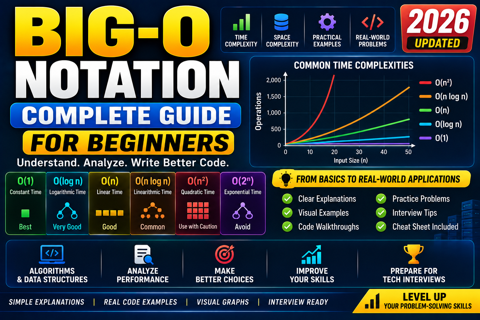
Big-O measures how runtime (or memory) scales with input size, not seconds. Learn the 7 common values in order from fastest to slowest: O(1) → O(log n) → O(n) → O(n log n) → O(n²) → O(2^n) → O(n!). Memorize the Big-O of Python list, dict, and set operations. For interviews, aim for O(n) or O(n log n) solutions; anything O(n²) or worse gets pushed back. Master this and 90 percent of “why is my code slow” questions answer themselves.
What Big-O actually measures (and what it does not)
Big-O describes the upper bound of how an algorithm grows as input size grows. It does not measure milliseconds. It ignores constants and lower-order terms so you can compare algorithms on a hardware-independent basis.
Example: two algorithms both process a list of n items. Algorithm A takes exactly n operations. Algorithm B takes 3n + 100 operations. On paper Algorithm B looks slower, but Big-O calls both O(n) because as n grows toward infinity, the coefficient 3 and the constant 100 stop mattering. This is the “why” behind every Big-O simplification rule.
What Big-O does NOT tell you: which algorithm is faster on your specific hardware, whether cache-friendliness matters for your data size, or how much memory the algorithm allocates (that is space complexity, covered below). Real-world performance always requires benchmarking on top of Big-O analysis.
The 7 most common Big-O classes (fastest to slowest)
| Big-O | Name | Example | n=1,000 |
|---|---|---|---|
| O(1) | Constant | Dict lookup, array index access | 1 op |
| O(log n) | Logarithmic | Binary search on sorted list | 10 ops |
| O(n) | Linear | Loop through a list once | 1,000 ops |
| O(n log n) | Linearithmic | Efficient sorting (mergesort, timsort) | 10,000 ops |
| O(n²) | Quadratic | Nested loop over the same list | 1 million ops |
| O(2^n) | Exponential | Naive recursive Fibonacci | 10^301 (infeasible) |
| O(n!) | Factorial | Traveling salesman brute force | infeasible past n=15 |
The right column tells the real story. O(1) and O(log n) are essentially free. O(n log n) is your daily “sort a list” workhorse. O(n²) becomes painful past ~10,000 items. O(2^n) and O(n!) are only viable for tiny inputs (n under 25 or so).
Real Python examples for each class
O(1) constant time:
def get_first(items):
    return items[0]           # index access, always 1 step

user_lookup = {"alice": 1, "bob": 2}
def find_user(name):
    return user_lookup.get(name)   # dict get, avg O(1)
O(log n) logarithmic time (binary search):
def binary_search(sorted_items, target):
    lo, hi = 0, len(sorted_items) - 1
    while lo <= hi:
        mid = (lo + hi) // 2
        if sorted_items[mid] == target:
            return mid
        elif sorted_items[mid] < target:
            lo = mid + 1
        else:
            hi = mid - 1
    return -1
# Each iteration halves the search space: 1000 items -> ~10 iterations
O(n) linear time:
def sum_items(items):
    total = 0
    for item in items:
        total += item
    return total
# One loop through n items = n operations = O(n)
O(n log n) linearithmic (built-in sort):
def sort_items(items):
    return sorted(items)      # Python's Timsort is O(n log n)
O(n²) quadratic (nested loop):
def has_duplicate_slow(items):
    for i in range(len(items)):
        for j in range(i + 1, len(items)):
            if items[i] == items[j]:
                return True
    return False
# Comparing every pair = n * n / 2 = O(n²)
O(2^n) exponential (naive Fibonacci):
def fib(n):
    if n <= 1:
        return n
    return fib(n - 1) + fib(n - 2)
# Each call spawns 2 more calls: 2^n total operations
# fib(50) = ~1 quadrillion calls, never finishes on a laptop
Fix Fibonacci with memoization or iteration and complexity drops to O(n). This is a classic dynamic programming setup you will meet again in Batch 11-C.
Big-O of Python built-in operations
Memorize these. They come up in every interview and every performance debugging session:
| Data structure | Access | Search | Insert | Delete |
|---|---|---|---|---|
| list (array) | O(1) | O(n) | O(n) | O(n) |
| dict (hashmap) | O(1) avg | O(1) avg | O(1) avg | O(1) avg |
| set (hashset) | n/a | O(1) avg | O(1) avg | O(1) avg |
| deque (linked list) | O(n) | O(n) | O(1) at ends | O(1) at ends |
| tuple | O(1) | O(n) | immutable | immutable |
Key insight: if you find yourself searching a list often, switch to a set or dict. Same code, but every lookup drops from O(n) to O(1). The single biggest performance win most Python beginners discover.
Big-O of common sorting algorithms
| Algorithm | Best | Average | Worst | Space |
|---|---|---|---|---|
| Bubble sort | O(n) | O(n²) | O(n²) | O(1) |
| Insertion sort | O(n) | O(n²) | O(n²) | O(1) |
| Merge sort | O(n log n) | O(n log n) | O(n log n) | O(n) |
| Quick sort | O(n log n) | O(n log n) | O(n²) | O(log n) |
| Timsort (Python) | O(n) | O(n log n) | O(n log n) | O(n) |
Python's sorted() and list.sort() use Timsort, a hybrid of merge sort + insertion sort tuned for real-world data. It hits O(n) on already-sorted or nearly-sorted input. That is why calling sorted() on data you just sorted is almost free.
How to calculate Big-O of your own code (5 rules)
- Drop constants. 3n becomes O(n). 500 becomes O(1). Constants do not matter as n grows.
- Drop lower-order terms. n² + n + 5 becomes O(n²). The dominant term wins as n grows large.
- Sequential steps add. A loop of n followed by a loop of m is O(n + m). If m and n are comparable, simplify to O(n).
- Nested loops multiply. A loop of n inside a loop of n is O(n × n) = O(n²).
- Recursive calls: count the tree. If each call spawns 2 recursive calls with depth n, it is O(2^n). If each call halves the input with 1 recursive call, it is O(log n).
Common mistakes when learning Big-O
- Confusing Big-O with actual runtime. O(n) is not "n seconds" or "n milliseconds." It is a scaling class. Actual runtime depends on hardware, cache, JIT, GC.
- Ignoring the "average" vs "worst" case. Quick sort is O(n log n) average but O(n²) worst case. Hash tables are O(1) average but O(n) worst case. In interviews, always state which case you are analyzing.
- Not counting hidden operations.
list.count(x)is O(n),x in some_listis O(n),list.insert(0, x)is O(n). Slice operations copy:my_list[1:]is O(n). - Overcomplicating simple loops.
for x in range(0, n, 2)is O(n), not O(n/2). The step size is a constant, dropped. - Trusting cheat sheets blindly. Cheat sheets show algorithmic complexity, but Python's specific implementation may differ. Check the official CPython docs when performance matters.
Big-O in coding interviews (what interviewers listen for)
The FAANG and top-tier interview loop expects you to:
- State the complexity out loud after each solution. "This is O(n) time, O(1) space" tells the interviewer you know what you built.
- Aim for O(n) or O(n log n) on medium-difficulty problems. If you land on O(n²), verbally acknowledge it and offer to optimize.
- Show the tradeoff. Using extra memory to trade O(n²) time for O(n) time is a classic move. Say "we can trade space for time by using a hashmap here."
- Avoid nested loops when a hashmap works. The "two sum" problem is the textbook example: O(n²) with nested loops, O(n) with a hashmap.
- Know your language's built-ins. Python
setoperations, JavaHashMap, JavaScriptMapandSet. These are your O(1) tools.
Official documentation
Frequently Asked Questions
Is O(1) always faster than O(n)?
For large n, yes. For small n (say, n under 20), the constant factors hidden by Big-O may make O(n) faster than O(1) with a large constant. Real example: Python dict lookup is O(1) but has more overhead than a simple 5-item list scan. Always benchmark when performance matters at your specific scale.
What is the difference between Big-O, Big-Omega, and Big-Theta?
Big-O is the upper bound (worst case scaling). Big-Omega (Ω) is the lower bound (best case). Big-Theta (Θ) is the tight bound when upper and lower match. In interviews you almost always say "Big-O" for anything you mean. Only formal computer science courses distinguish rigorously.
Does Big-O apply to space or only time?
Both. Space complexity measures memory used. An algorithm that allocates a new array of size n has O(n) space. An in-place algorithm has O(1) space. Recursive algorithms use O(depth) space for the call stack. Modern interviews often ask for both time AND space Big-O of your solution.
Why is binary search O(log n) and not O(n/2)?
Each step of binary search halves the search space. After k steps, only n / 2^k items remain. The algorithm stops when 1 item remains, so we solve 2^k = n for k, giving k = log₂ n. That is O(log n). The "log" in Big-O is base-2 by convention but any log base differs only by a constant factor (which Big-O drops).
How do I get better at analyzing Big-O quickly?
Practice on LeetCode Easy problems and always state the complexity after each. Read solutions and check whether the author's stated complexity matches yours. Do this for 30-50 problems and Big-O analysis becomes automatic. The Sedgewick or CLRS textbook offers rigorous depth if you want the formal side.
Which Big-O should I aim for in a coding interview?
Aim for the optimal solution the problem allows. Most string/array problems have O(n) or O(n log n) optimal solutions. Graph problems are typically O(V + E). Dynamic programming problems are typically O(n × m). If your first solution is O(n²) and you know a hashmap can drop it to O(n), verbalize the improvement even if you do not have time to code it, that scores partial credit.
Related DSA + Interview tutorials
- DSA Roadmap for BSIT Students 2026 (coming this week)
- Recursion Explained with Real Examples 2026 (coming this week)
- Sorting Algorithms Cheat Sheet 2026 (coming this week)
- Top 100 Coding Interview Questions 2026 (coming next week)
Official documentation
- Python.org: TimeComplexity of built-in operations
- Big-O Cheat Sheet (data structures + sorting)
- Python.org: collections.deque and OrderedDict

Adones Evangelista
Programmer & Technical Writer at PIES IT Solution
Adones Evangelista is a programmer and writer at PIES IT Solution, author of over 900 tutorials and error-fix guides at itsourcecode.com. Specializes in JavaScript, Django, Laravel, and Python error debugging covering ValueError, TypeError, AttributeError, ModuleNotFoundError, and RuntimeError, plus C/C++ and PHP capstone projects for BSIT students.
Expertise: JavaScript · Python · Django · Laravel · Error Debugging · C/C++ · View all posts by Adones Evangelista →