Parts of Excel Window 2026: Complete Guide with Labeled Diagram [Free PDF]

Q: What are the different parts of an Excel window?

The main parts of an Excel window are: Title Bar, Quick Access Toolbar, Ribbon, Name Box, Formula Bar, Worksheet Area, Sheet Tabs, Status Bar, Scroll Bars, and View Buttons with Zoom Control. Each serves a distinct function — the Ribbon holds commands by tab, the Name Box shows the active cell address, the Formula Bar displays and edits cell content, and the Worksheet Area is the grid of cells where data is entered.

Q: What are the 4 major parts of Excel?

The 4 major components of Excel are: (1) Cells — basic units identified by column letter + row number; (2) Rows and Columns — horizontal rows (numbered) and vertical columns (lettered) forming the grid; (3) Worksheets — individual tabs within a workbook; (4) Formulas and Functions — calculations like SUM, AVERAGE, and VLOOKUP that process cell data automatically.

Q: What is the difference between a workbook and a worksheet in Excel?

A workbook is the entire Excel file (.xlsx) that can contain multiple worksheets. A worksheet (sheet or tab) is a single spreadsheet inside a workbook. When you open Excel, you have one workbook with one worksheet named Sheet1 by default. Each worksheet has its own grid of cells and operates independently, though formulas can reference cells across worksheets.

Q: What is the Ribbon in Excel and what does it do?

The Ribbon is the wide tabbed toolbar at the top of Excel that groups commands by purpose. Tabs include Home, Insert, Page Layout, Formulas, Data, Review, View, and contextual tabs for charts and objects. The Ribbon replaced the old menu-and-toolbar system in Excel 2007. You can minimize it with Ctrl+F1 or hide it completely via the Ribbon Display Options.

Q: What is the formula bar used for in Excel?

The formula bar displays the actual content of the selected cell and lets you type or edit it. When a cell contains a formula, the cell shows the result while the formula bar shows the formula itself. This makes the formula bar the primary place to write, audit, and fix formulas. Expand it for multi-line formulas by dragging its bottom border or pressing Ctrl+Shift+U.

Q: What is the Name Box in Excel?

The Name Box is the small box to the left of the formula bar showing the active cell address. It has three uses: navigate to any cell by typing its address, select ranges by typing a range like A1:D10, and create named ranges by typing a custom name for selected cells. Named ranges make formulas more readable, like using SUM(SalesData) instead of SUM(B2:B500).

Q: What is the Quick Access Toolbar in Excel?

The Quick Access Toolbar (QAT) is a small customizable bar above or below the Ribbon with one-click shortcuts to favorite commands. By default it includes Save, Undo, and Redo. You can add any Ribbon command by right-clicking it and choosing Add to Quick Access Toolbar. Customize via File → Options → Quick Access Toolbar for productivity wins.

Q: How do I show or restore the Ribbon if it's hidden?

Press Ctrl+F1 to toggle the Ribbon back. Or click the small arrow icon at the top-right of Excel and choose Show Tabs and Commands. In Excel 365, the option is Always show Ribbon under Ribbon Display Options. If the entire Ribbon including tabs is missing, your Excel may be in Auto-hide mode — click the top edge of the window to reveal it.

Q: Why is the formula bar missing in my Excel?

The formula bar can be hidden via the View tab. To restore it: go to View tab → Show group and check the Formula Bar checkbox. Or go to File → Options → Advanced, scroll to Display, and check Show formula bar. The formula bar can also be collapsed to one row — drag its bottom edge down to expand it. If still missing, try Repair Office via Control Panel.

Q: What is the difference between rows and columns in Excel?

Rows run horizontally and are numbered (1, 2, 3, …) along the left side. Columns run vertically and are lettered (A, B, C, …) along the top. Their intersection is a cell, identified by column letter + row number (e.g., C5). Modern Excel supports 1,048,576 rows and 16,384 columns per worksheet. Use rows for records and columns for fields — the standard sortable/filterable data layout.

This tutorial will provide a complete guide to different parts of the Excel window. It is designed to help you become an expert in no time.

If you like these types of tutorials, we also have Identifying different parts of a Microsoft Word window and different parts of a PowerPoint window with its functions.

What is Excel?

Excel is a powerful spreadsheet program that is widely used for data analysis, reporting, and budgeting.

This software is highly versatile and offers a wide range of features to meet the needs of both casual and professional users.

A little recap, Excel is a spreadsheet software developed by Microsoft that is part of the Microsoft Office suite.

It was first released in 1985 and has since evolved into a powerful tool for data analysis, reporting, and budgeting.

Besides that, this software allows us to create, edit, and save spreadsheets that can contain numerical data, text, and formulas.

Now, let’s get in-depth and understand the different parts of Excel…

Identifying Different Parts of Excel Window

Every time we open Excel, we are presented with the Excel window. The Excel window consists of several parts, each with a specific purpose.

Understanding these parts is essential to effectively use Excel.

Hence, take a look at the image below as we tackle definitions and functions as we go along.

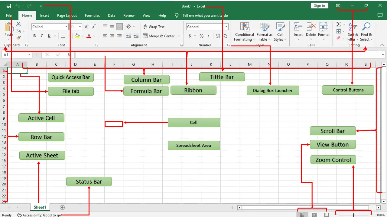
Here are the parts of Excel along with each function.

The Ribbon

The Ribbon is located at the top of the Excel window and provides access to the most commonly used Excel commands.

The ribbon is composed of the following:

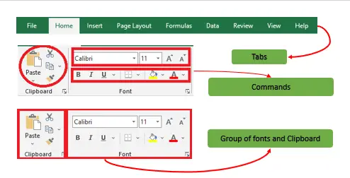
Groups
They organize related commands; the name of each group is displayed below the Ribbon.
Commands
They appear within each group, as previously stated.
Tabs
They are the Ribbon’s top part, and they include groups of related commands.

Some of the tabs that you may see in the ribbon include:

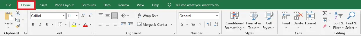
Home
- Basically, the Home tab contains commands for formatting cells, working with fonts, applying styles, and more.

Insert
- The Insert tab allows you to insert different elements into your worksheet, such as charts, tables, shapes, and images

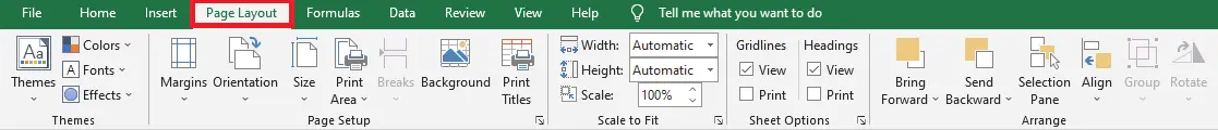
Page Layout
- Page layout tab provides options for controlling the overall appearance of your worksheet, such as setting margins, paper size, and page orientation.

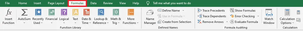
Formulas
- This Formula tab contains commands for working with formulas and functions, such as creating and editing formulas, using functions, and managing named ranges.

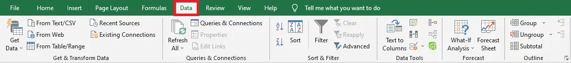
Data
- This Data tab provides commands for working with data, such as sorting, filtering, and grouping data.

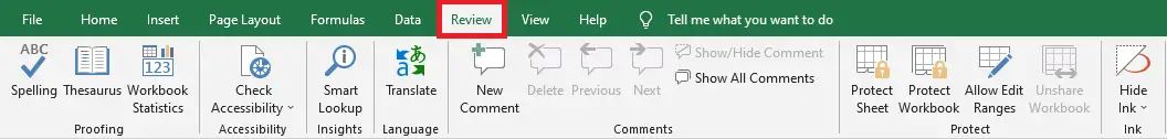
Review
- Review tab provides commands for reviewing and commenting on your worksheet, such as checking spelling and grammar, tracking changes, and inserting comments.

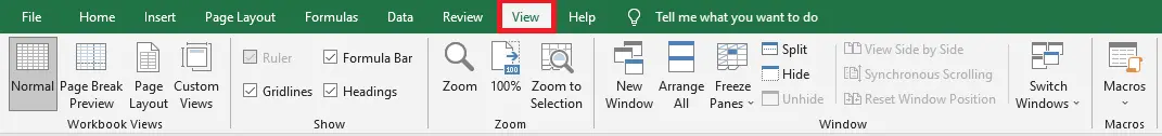
View
- This view tab provides commands to view the Excel worksheet, like changing views, freeze panes, arranging multiple windows, etc.

Quick Access Toolbar

This toolbar can be found in the upper left-hand corner of the screen.

Its purpose is to display the most frequently used Excel commands.

You can personalize this toolbar with your preferred commands.

File Tab

This File menu does the file-related operations wherein you can create a new Excel workbook, open an existing file, save, save as, print file, etc.

Title Bar

The header or title bar of the spreadsheet is located at the top of the window. It presents the name of the active document.

Control buttons

They are those symbols in the upper-right of the window that allow you to modify the labels, minimize, maximize, share, and close the sheet.

Cells

Cells are those parallelepipeds that divide the spreadsheet into several segments that allow rows to be separated from columns.

The first cell of a spreadsheet is represented by the initial letter of the alphabet and the number one (A1).

Active Cell

The cell is selected in the active worksheet.

Dialog Box Launcher

This is a very small down arrow located in the lower-right corner of a command group on the Ribbon.

By clicking this arrow explore more options about the concerned group.

Name box

The Name Box is located to the left of the formula bar and displays the cell address of the active cell.

You can also use it to quickly navigate to a specific cell in your worksheet by typing its address.

Formula bar

It is a bar that allows you to observe, insert, or edit the information/formula entered in the active cell.

Scrollbars

Those are the tools that allow you to mobilize both the vertical and horizontal view of the document.

They can be activated by clicking on the internal bar of your platform, or on the arrows, you have on the sides.

In addition to that, you can use the mouse wheel to automatically scroll up or down; or use the directional keys.

Spreadsheet Area

This is the area where you enter your data. It is the entire spreadsheet, complete with rows, cells, columns, and built-in data.

We can carry out toolbar activities or arithmetic operation formulas using shortcuts.

The blinking vertical bar called “cursor” is the insertion point. It indicates the insertion location of the typing.

The Worksheet

The Worksheet is where you enter and manipulate data in Excel.

It is made up of rows and columns and is where you enter and format data, create formulas, and build charts.

In addition to that, the worksheet is the main working area in Excel and is where you will spend most of your time.

The Formula Bar

The Formula Bar is located above the worksheet and is used to enter and display formulas.

When you click on a cell in the worksheet, the contents of that cell are displayed in the Formula Bar.

You can also use the Formula Bar to enter or edit formulas.

The Status Bar

The status bar is located at the bottom of the Excel window and provides information about the current state of your worksheet.

View Buttons

It is a group of three buttons arranged at the left of the Zoom control, close to the right-bottom of the screen.

Through this, you can see three different types of Excel sheet views.

Normal view: This displays the Excel page in normal view.
Page Layout view: This displays the exact view of Excel’s page as it will be printed.
Page Break view: This shows the page break preview before printing.

Zoom Control

The Zoom control in Microsoft Excel is a feature that allows you to change the magnification level of your worksheet.

By using the zoom control, you can make the content of your worksheet appear larger or smaller on the screen.

What are the 4 Major Parts of Excel?

Microsoft Excel is a powerful spreadsheet software that consists of several different parts, but the four major components are:

Cells

This is the basic unit of an Excel worksheet, where data is entered and processed. Cells are organized into rows and columns, creating a grid-like structure.

Rows VS Columns

Rows are horizontal lines that run across the worksheet and are identified by numbers, while columns are vertical lines that run down the worksheet and are identified by letters.

Worksheets

A worksheet is a single sheet within a workbook, which is the main document in Excel.

You can have multiple worksheets within a workbook, and each worksheet can contain different data and calculations.

Formulas and Functions

These are mathematical expressions that can perform calculations based on the data in the cells.

Functions are predefined formulas that perform specific calculations, such as SUM or AVERAGE, while formulas are custom expressions that you can create.

These four components form the foundation of Microsoft Excel and are used to manage, analyze, and visualize data.

What is the difference between a Worksheet and a Workbook in Excel?

A worksheet is a single sheet in an Excel workbook, while a workbook is a collection of one or more worksheets.

Each worksheet in a workbook is represented by a tab at the bottom of the Excel window.

Frequently Asked Questions

What are the different parts of an Excel window?

The main parts of an Excel window are: (1) Title Bar — shows the workbook name at the top; (2) Quick Access Toolbar — customizable shortcuts above the Ribbon; (3) Ribbon — tabbed command interface (Home, Insert, Page Layout, etc.); (4) Name Box — shows the active cell address; (5) Formula Bar — where you type or edit cell content; (6) Worksheet Area — the grid of cells; (7) Sheet Tabs — switch between worksheets; (8) Status Bar — shows mode, calculations, view buttons at the bottom; (9) Scroll Bars — navigate large worksheets; (10) View Buttons + Zoom Control — change view type and zoom level.

What are the 4 major parts of Excel?

The 4 major components of Excel are: (1) Cells — the basic units where data is entered, identified by column letter + row number (e.g., A1, B5); (2) Rows VS Columns — rows run horizontally (numbered 1, 2, 3…), columns run vertically (lettered A, B, C…); together they form the grid; (3) Worksheets — individual tabs within a workbook, each a separate spreadsheet; (4) Formulas and Functions — calculations and built-in operations (SUM, AVERAGE, VLOOKUP) that process cell data automatically.

What is the difference between a workbook and a worksheet in Excel?

A workbook is the entire Excel file (.xlsx) — it can contain multiple worksheets. A worksheet (also called a sheet or tab) is a single spreadsheet inside a workbook with rows and columns of cells. When you open Excel, you open one workbook by default with one worksheet named “Sheet1.” You can add more worksheets via the + icon next to sheet tabs. Each worksheet has its own grid (1,048,576 rows × 16,384 columns in modern Excel) and operates independently — though formulas can reference cells across worksheets.

What is the Ribbon in Excel and what does it do?

The Ribbon is the wide tabbed toolbar at the top of Excel that groups all commands by purpose. Tabs include Home (formatting, clipboard), Insert (charts, tables, images), Page Layout (margins, themes), Formulas (function library), Data (sorting, filtering, import), Review (spelling, protection), View (zoom, freeze panes), and contextual tabs that appear when you select objects like charts. The Ribbon replaced the old menu-and-toolbar system in Excel 2007 and has been the standard interface ever since. You can minimize it (Ctrl+F1) to show only tab names, or hide it completely.

What is the formula bar used for in Excel?

The formula bar displays the actual content of the selected cell and lets you type or edit it. If a cell contains a formula like =SUM(A1:A10), the cell shows the result (e.g., 250) but the formula bar shows the formula itself. This makes the formula bar the primary place to write, audit, or fix formulas. You can also use it for long text entries that don’t fit visibly in the cell. To expand the formula bar for multi-line formulas, drag its bottom border down or press Ctrl+Shift+U.

What is the Name Box in Excel?

The Name Box is the small box to the left of the formula bar that shows the address of the currently selected cell (e.g., “B7”). It has three main uses: (1) Navigate — type any cell address (e.g., “Z500”) and press Enter to jump there instantly; (2) Select ranges — type a range like “A1:D10” to select all those cells; (3) Name ranges — type a custom name (like “SalesData”) for a selected range to reuse in formulas. Named ranges make complex formulas readable: =SUM(SalesData) beats =SUM(B2:B500).

What is the Quick Access Toolbar in Excel?

The Quick Access Toolbar (QAT) is a small customizable bar above or below the Ribbon with one-click shortcuts to your most-used commands (Save, Undo, Redo by default). You can add any command — right-click any Ribbon button and choose “Add to Quick Access Toolbar.” This is a major productivity boost in Excel 365 because you can keep favorites like Sort, Filter, Format Painter, and Paste Special always one click away regardless of which Ribbon tab is active. Customize via File → Options → Quick Access Toolbar.

How do I show or restore the Ribbon if it’s hidden?

If the Ribbon disappears, press Ctrl+F1 to toggle it back. Or click the small arrow icon at the top-right corner of Excel and choose “Show Tabs and Commands” to fully restore it. In Excel 365, the option is labeled “Always show Ribbon” under the Ribbon Display Options dropdown (top-right). If the entire Ribbon is missing including tabs, your Excel window may be in Auto-hide mode — click the top edge of the Excel window to reveal it temporarily, then change the display option.

Why is the formula bar missing in my Excel?

The formula bar can be hidden via the View tab. To restore: go to View tab → Show group and check the “Formula Bar” checkbox. If that doesn’t work, go to File → Options → Advanced and scroll to the “Display” section — make sure “Show formula bar” is checked. The formula bar can also be collapsed to one row — drag its bottom edge down to expand it back to multiple rows. If it’s still missing after these steps, your Excel may have a corrupted Ribbon — try Repair Office via Control Panel → Programs → Microsoft Office → Change → Repair.

What is the difference between rows and columns in Excel?

Rows run horizontally and are numbered (1, 2, 3, …) along the left side of the worksheet. Columns run vertically and are lettered (A, B, C, …) along the top. The intersection of a row and column is a cell, identified by its column letter + row number (e.g., C5 = column C, row 5). Modern Excel supports 1,048,576 rows and 16,384 columns per worksheet (column XFD is the last). Use rows for records/entries (one customer per row) and columns for fields/attributes (Name, Email, Sales) — this is the standard layout for sortable, filterable data.

Conclusion

Finally, this tutorial identifying Parts of an Excel Window provides you with an idea of what function you will use in your worksheet.

Now that you understand the components and functions of Excel Windows, you are ready to move on to more advanced Excel functions.

Excel 365 vs Excel 2019: What Changed in the Interface?

If you’re moving from Excel 2019 (or older) to Excel 365 (Microsoft 365 subscription), several interface elements look different. Here’s what to expect:

The Search Box replaces “Tell Me”

The old “Tell Me what you want to do” box at the top of the Ribbon is now a full Microsoft Search box. It searches commands, files, recent actions, and Microsoft Help — much more powerful than the original “Tell Me” feature.

Dynamic Arrays change the formula experience

Excel 365 introduced dynamic arrays — formulas like =SORT(A1:A10) now “spill” results into multiple cells automatically. The formula bar shows the formula in only one cell (the anchor), and the spilled cells show “ghost” formulas you can’t directly edit. This is a major shift from Excel 2019 which required Ctrl+Shift+Enter array formulas.

New chart and PivotTable types

Excel 365 includes chart types not available in 2019: Funnel charts, Map charts, and improved PivotChart interactivity. The Insert tab shows these in the Charts group.

Modern data connections

Excel 365’s Data tab has expanded “Get & Transform Data” (Power Query) capabilities, with connectors to cloud sources like SharePoint, Salesforce, and OData feeds — most of these were add-ins in Excel 2019.

AI-assisted features (2026 update)

Excel 365 in 2026 includes Copilot integration on the Home tab. The Copilot pane appears as a sidebar where you can ask natural language questions about your data (“show me sales trends by region”) and Excel generates the formula, chart, or PivotTable for you. This is the biggest interface addition since the Ribbon itself.

What stayed the same

The core interface — Ribbon, Name Box, Formula Bar, Worksheet area, Sheet tabs, Status Bar — is identical in layout. Learning Excel 2019 layout still applies to Excel 365 95%+ of the time.

Essential Excel Keyboard Shortcuts for Each Interface Section

Mastering shortcuts for each interface section turns Excel from a clicking exercise into a fluid workflow. Here are the most useful shortcuts mapped to the Excel window components covered above:

Ribbon & Quick Access Toolbar shortcuts

Alt — display KeyTips (letter overlays) for every Ribbon tab and QAT button. Press the letter to activate that command.
Ctrl+F1 — toggle Ribbon visibility (show/hide)
Alt+F+T — open Excel Options dialog (where you customize QAT, etc.)
Alt+1, Alt+2, Alt+3, … — activate QAT items 1, 2, 3, etc. in order

Formula Bar & Name Box shortcuts

F2 — edit the active cell (cursor jumps into the formula bar)
Ctrl+Shift+U — expand/collapse the formula bar to multi-line view
F3 — open “Paste Name” dialog to insert a named range
Ctrl+G or F5 — Go To dialog (jump to any cell or named range, alternative to Name Box)

Worksheet & Sheet Tab shortcuts

Ctrl+Page Down / Page Up — switch to next / previous worksheet tab
Shift+F11 — insert a new worksheet
Alt+Shift+F1 — rename the current worksheet (older method) / right-click tab → Rename
Ctrl+Home — jump to cell A1
Ctrl+End — jump to the last used cell in the worksheet
Ctrl+Arrow keys — jump to the edge of data in any direction

Status Bar & View shortcuts

Ctrl+F2 — print preview (or jump to View tab depending on version)
Alt+W, Q — open Zoom dialog
Alt+W, V, G — toggle gridlines
Ctrl+Shift+L — toggle filter on selected range (the AutoFilter dropdowns appear)

Most BSIT students never learn these shortcuts and spend 2-3x longer than necessary on simple tasks. Pick 5 shortcuts a week and practice — within a month you’ll dramatically speed up your Excel workflow.

Common Excel Interface Problems and Quick Fixes

If parts of your Excel window vanish or behave unexpectedly, here’s how to restore them quickly:

The Ribbon disappeared

Quick fix: Press Ctrl+F1 to toggle the Ribbon back. If only tab names are visible without commands, the Ribbon is collapsed — click any tab name once to temporarily show, or click the pin icon at the bottom-right of the Ribbon to keep it pinned. In Excel 365, use the Ribbon Display Options arrow at the top-right and choose “Always show Ribbon.”

The Formula Bar is missing

Quick fix: Go to View tab → Show group → check “Formula Bar”. If that checkbox is greyed out, go to File → Options → Advanced → Display → check “Show formula bar”. The formula bar may also be collapsed to one row — drag its bottom edge down to expand.

The Status Bar at the bottom is gone

Quick fix: Right-click the bottom of the Excel window. If the right-click menu appears, the status bar is just below the visible area — drag the Excel window to a larger size or maximize. If no menu appears, restart Excel (sometimes the status bar gets stuck after a crash).

Sheet Tabs are missing at the bottom

Quick fix: Go to File → Options → Advanced → scroll to “Display options for this workbook” → check “Show sheet tabs”. If still missing, the horizontal scroll bar may be covering them — drag the scroll bar resize handle (the small dots between scroll bar and sheet tabs) to the right.

Cells appear shifted or wrong size

Quick fix: Press Ctrl+0 (zero) to hide selected columns, or Ctrl+Shift+0 to unhide them. To reset zoom: View tab → Zoom group → 100%. To reset frozen panes: View tab → Freeze Panes → Unfreeze Panes.

The Name Box won’t accept input

Quick fix: You’re probably in edit mode on a cell. Press Esc to exit cell editing, then click the Name Box. If you still can’t type, the Excel window may have lost focus — click any cell first, then click the Name Box.

Excel ribbon shortcut letters (KeyTips) don’t appear

Quick fix: Press and release Alt, then wait 1 second. If they still don’t show, Excel may have a stuck modifier key — press Esc a few times to reset, then try Alt again. If persistent, restart Excel.

For deeper Excel troubleshooting beyond interface issues, browse our complete Excel tutorial series.

What is Excel?

Identifying Different Parts of Excel Window

The Ribbon

Quick Access Toolbar

File Tab

Title Bar

Control buttons

Cells

Active Cell

Dialog Box Launcher

Name box

Formula bar

Scrollbars

Spreadsheet Area

The Worksheet

The Formula Bar

The Status Bar

View Buttons

Zoom Control

What are the 4 Major Parts of Excel?

Cells

Rows VS Columns

Worksheets

Formulas and Functions

What is the difference between a Worksheet and a Workbook in Excel?

Frequently Asked Questions

Conclusion

Excel 365 vs Excel 2019: What Changed in the Interface?

The Search Box replaces “Tell Me”

Dynamic Arrays change the formula experience

New chart and PivotTable types

Modern data connections

AI-assisted features (2026 update)

What stayed the same

Essential Excel Keyboard Shortcuts for Each Interface Section

Ribbon & Quick Access Toolbar shortcuts

Formula Bar & Name Box shortcuts

Worksheet & Sheet Tab shortcuts

Status Bar & View shortcuts

Common Excel Interface Problems and Quick Fixes

The Ribbon disappeared

The Formula Bar is missing

The Status Bar at the bottom is gone

Sheet Tabs are missing at the bottom

Cells appear shifted or wrong size

The Name Box won’t accept input

Excel ribbon shortcut letters (KeyTips) don’t appear

Looking for similar projects or tutorials?

Leave a Comment Cancel reply

Quick Links

Top Categories

Get Free Capstone Resources