
What is a Pivot Table in Excel?
A pivot table in Excel allows you to arrange data in various ways with just a few clicks.
It automatically analyzes, summarizes, sorts, and filters a huge amount of data.
As well as it calculates the total and average of the data and presents the results in a reasonable manner.
Apart from that, users can easily compare data from different perspectives.
These are the characteristics and a pivot table capable of:
- Sort and visualize huge amounts of data in a user-friendly way.
- It summarizes data by categories and subcategories.
- Pivoting enables to rotation of rows and columns to visualize different summaries of the presented data.
- It presents the subtotal and aggregate numerical data in your worksheet.
- The level of data expands and collapses and digs down to see the details behind any total.
- Output concise and engaging online data or printed reports.
How to make and use a pivot table in Excel
A pivot table Excel is easy to make and use; you just have to follow the following guide:
Using a Recommended Pivot Tables
- Create and organize your data into rows and columns. If you already have one, then proceed to step 2.
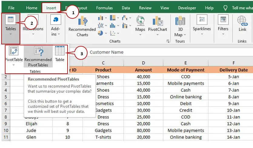
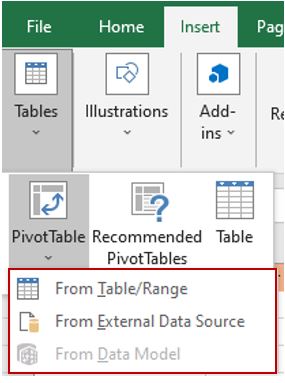
- Click on the “Insert” tab in the menu bar.
- In the “Tables” group, click “Recommended Pivot Tables” or “PivotTable.”
When we click “Recommended Pivot Tables,” this is what it looks like.
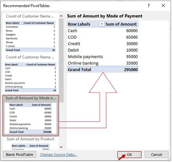
4. You can choose different types of pivot tables; in our case, we chose “Sum of Amount by Mode of Payment.“
5. Then click the “OK” button.
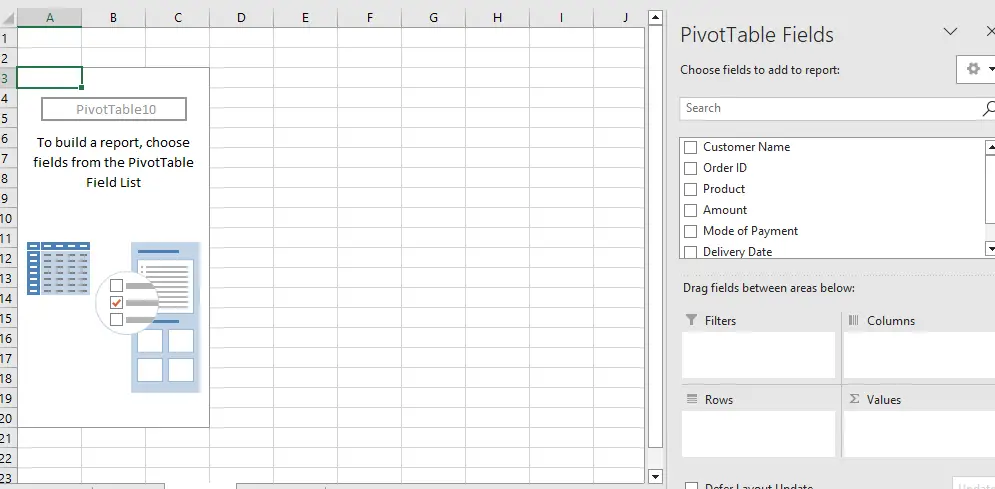
6. After we click the “OK” button, it will create the pivot table in a new worksheet, as you can see in the image below.
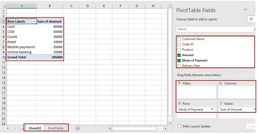
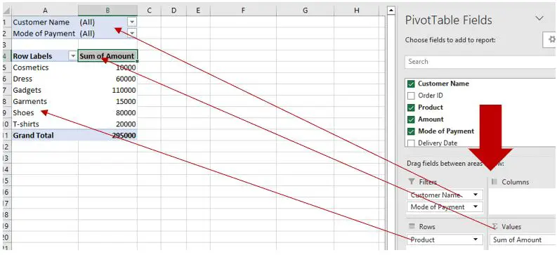
7. On the right side, you can customize your pivot table. You can add more data under “Drag fields between areas below:” You can drag the data below, just like what you can see in our example below:
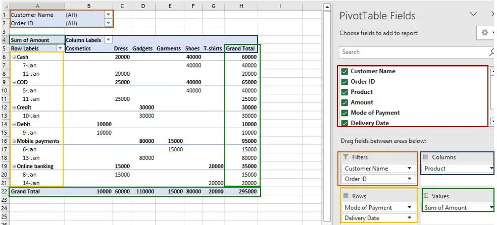
As you can see, we drag different data sets with matching colors so that it is easy for you to identify each data point in the pivot table.
Note: If this is your first time using a pivot table, this "Recommended Pivottable" is the best choice for you. It offers different types of pivot tables, which you may use.
Kindly check the video below:
The video contains instructions for creating a pivot table, an example of how to arrange and sort, and how to drag and drop fields in the layout section using the mouse.
2. Using a Pivot Table
If we click the drop-down menu of the pivot table, it looks like this:
Note: You can just click the PivotTable, and it will display the "PivotTable from the table or range." If you don't like to click the drop-down menu of PivotTable, that's fine.
When you click “From Table/Range” it will show a dialog box that you’ll see below:
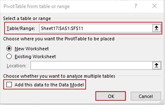
- You can choose the table or range that you want and where you want the pivot table to be placed.
- And, if you want to analyze multiple tables, just check the checkbox.
- Then click the “OK” button, and it will open a new worksheet.
4. A new worksheet will appear, and you can drag the data that you want to see in the pivot table into the “Drag fields between areas below:”
Kindly check the video below:
5. Alternatively, if you want to show each customer’s order, you just have to sort each name so that you’ll see their order. Refer to the video below:
Adding a field to the Pivot Table
In order to add it to the layout section, you just have to select the check box next to its field name in the Field section, or you can drag it to the Drag Fields section.
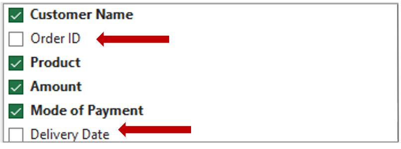
- In the row area, non-numerical fields are added to this.
- In the Values area, numeric fields are added to this.
- In the column area, date and time hierarchies are added to this.
- In the filters area, either non-numerical or numeric fields and date and time are okay to add; it just depends on your requirement.
Remove a field from a Pivot Table
There are a lot of ways to remove a field from your pivot table.
Using a right-click
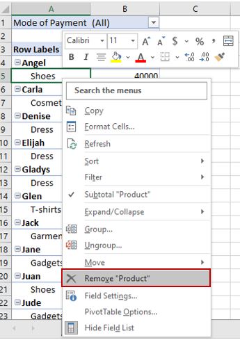
- Right-click the data in the layout section that you would like to remove.
- After you right-click, a pop-up menu appears. Select “Remove product.”
Note: In our case, "product" is what we wanted to remove, that is why "Remove product" is being displayed in the pop-up menu.
Drag to remove the field.
Kindly check the video below:
Different functions and calculations of a pivot table in Excel
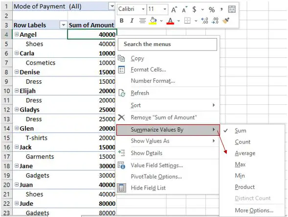
These are the functions of the pivot table:
- Sum calculates the sum of the values.
- Count counts the number of non-empty values (works as the COUNTA function).
- Average calculates the average of the values.
- Max finds the largest value.
- Min finds the smallest value.
- Product calculates the product of the values.
If you want more functions, click “More Options.” It will show the value field settings dialog box.
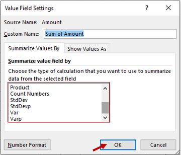
You can see in the image below the list of calculation options:
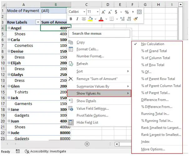
Note: The "Show values" option is just optional; it is not usually used by many unless if it is necessary.
Conclusion
This guide on how to make and use a pivot table in Excel is able to help you analyze and summarize data in a matter of minutes.
We hope that this guide was totally helpful to you and that you’ve learned new ideas with regard to how to use a pivot table in Excel.
Thank you very much for continuing to read until the end of this article. In case you have more questions, feel free to comment.

Caren Bautista
Technical Writer at PIES IT Solution
Responsible for crafting clear, well-structured, and beginner-friendly content across the platform. Handles the writing, proofreading, and editorial review of tutorials, guides, and documentation to ensure every article is accurate, readable, and easy to follow.
Expertise: Technical Writing · Content Creation · Documentation · Editorial Writing · JavaScript · TypeScript · Python · Python Errors · HTTP Errors · MS Excel · View all posts by Caren Bautista →