How to Use IF Function in Google Sheets (Nested + Advanced 2026)

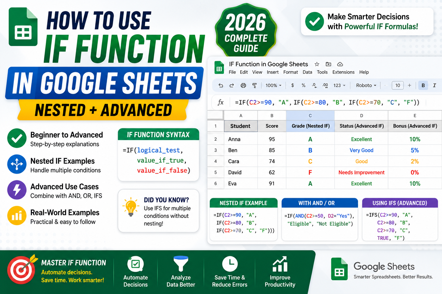
The IF function is the most useful conditional logic tool in Google Sheets. It lets you make decisions in formulas: “IF this cell is greater than 100, show YES, otherwise show NO.” From basic budget checks to complex classification systems, IF is the foundation. This 2026 guide walks through the basic syntax, nested IFs, the newer IFS function, and combining IF with AND/OR/NOT for real spreadsheet work.

Basic IF syntax

The IF function has three parts:

=IF(logical_test, value_if_true, value_if_false)

# Example: is the amount in A1 over 100?
=IF(A1>100, "Over budget", "OK")

Read as: “If A1 is greater than 100, return ‘Over budget’. Otherwise return ‘OK’.”

The logical test can use any comparison operator: >, <, >=, <=, =, <>.

Common single-IF examples

# Pass or fail based on a score
=IF(B2>=60, "Pass", "Fail")

# Apply a discount if quantity is 10 or more
=IF(C5>=10, D5*0.9, D5)

# Flag empty cells
=IF(E10="", "Missing", E10)

# Compare two cells
=IF(F3=G3, "Match", "Mismatch")

# Show absolute value with logic
=IF(H2<0, -H2, H2)

Nested IF (multiple conditions)

To handle more than two possible outcomes, nest IFs inside each other:

# Grade classification
=IF(A1>=90, "A",
  IF(A1>=80, "B",
    IF(A1>=70, "C",
      IF(A1>=60, "D", "F"))))

# Priority based on days overdue
=IF(B2>=30, "Critical",
  IF(B2>=14, "High",
    IF(B2>=7, "Medium", "Low")))

Google Sheets allows up to 128 levels of nesting, but readability drops fast beyond 3-4 nested IFs. For more complex logic, use the IFS function instead.

IFS (cleaner alternative to nested IFs)

IFS lets you write multi-branch logic more readably:

=IFS(
  condition1, value1,
  condition2, value2,
  ...
  TRUE, default_value
)

# Grade classification with IFS
=IFS(
  A1>=90, "A",
  A1>=80, "B",
  A1>=70, "C",
  A1>=60, "D",
  TRUE, "F"
)

The final TRUE condition is the catch-all default (like an "else" clause). Without it, IFS returns #N/A if no condition matches.

Combine IF with AND/OR

Use AND when ALL conditions must be true. Use OR when ANY condition being true is enough.

# Eligible if age is 18+ AND has valid ID
=IF(AND(A1>=18, B1="Yes"), "Eligible", "Not eligible")

# Weekend if Saturday OR Sunday
=IF(OR(WEEKDAY(A1)=1, WEEKDAY(A1)=7), "Weekend", "Weekday")

# Approve if score>80 AND (department=Sales OR Marketing)
=IF(AND(C1>80, OR(D1="Sales", D1="Marketing")), "Approve", "Review")

IF with NOT for negation

NOT flips a boolean condition:

# Flag rows that are NOT paid
=IF(NOT(A1="Paid"), "Outstanding", "")

# Alert if department is NOT one of the approved list
=IF(NOT(OR(B1="HR", B1="Legal", B1="Finance")), "Needs review", "OK")

NOT is often optional (you can use <> for not-equal), but it makes the intent clearer when combined with other functions.

IF with text and numbers

IF handles both text and number outputs. Combine with math for calculations:

# Bonus calculation: 10% if sales>1000, 5% otherwise
=IF(A1>1000, A1*0.10, A1*0.05)

# Show percentage as formatted text
=IF(B1=0, "No data", B1/C1*100 & "%")

# Concatenate text and number
=IF(D1>100, "Over by " & (D1-100) & " units", "Within limit")

IFERROR: catch and handle errors

Related to IF, IFERROR catches formula errors and returns a fallback:

# Divide but return "N/A" if divisor is zero
=IFERROR(A1/B1, "N/A")

# VLOOKUP but return blank if not found
=IFERROR(VLOOKUP(C1, D:E, 2, FALSE), "")

# Combine IF and IFERROR
=IFERROR(IF(A1>0, A1*100, "Negative"), "Error")

IFERROR is common in production spreadsheets to avoid #DIV/0!, #N/A, and #VALUE! errors leaking into reports.

Common IF pitfalls

• Text vs number comparison. IF("10">5, ...) may not work as expected because "10" is text. Use VALUE() to convert: IF(VALUE(A1)>5, ...).
• Case sensitivity in text comparison. IF(A1="Yes", ...) matches "Yes" but not "yes" or "YES". For case-insensitive match, use LOWER: IF(LOWER(A1)="yes", ...).
• Nested IFs get unwieldy fast. Once you hit 3+ nested IFs, switch to IFS or a VLOOKUP against a lookup table.
• Forgetting the FALSE branch. IF(A1>10, "Big") without a false value returns FALSE for anything not matching. Always include the third argument.
• Comparing empty cells. Empty cells match both "" and 0 in different situations. Test explicitly: IF(ISBLANK(A1), "Empty", A1).
• Using = for assignment instead of comparison. All formulas start with =. Inside an IF, use = only for comparison (never for assignment; there's no such thing in formulas).

When to use IF vs another function

• Simple two-outcome condition: use IF.
• 3-5 branches: use IFS for clarity.
• Many discrete values that map to outputs: use VLOOKUP or XLOOKUP against a lookup table.
• Count based on a condition: use COUNTIF or COUNTIFS.
• Sum based on a condition: use SUMIF or SUMIFS.
• Average based on a condition: use AVERAGEIF or AVERAGEIFS.

IF is the general-purpose tool. The specialized functions (COUNTIF, SUMIF, etc.) are cleaner when you're doing aggregation with a condition attached.

Practical example: expense classifier

Column A: expense category. Column B: amount. Column C: month.

# Flag high-priority expenses
=IF(AND(B2>1000, OR(A2="Travel", A2="Equipment")), "Requires approval", "Standard")

# Categorize expense size
=IFS(
  B2>=5000, "Major",
  B2>=1000, "Significant",
  B2>=100, "Standard",
  TRUE, "Small"
)

# Q4 alert
=IF(AND(MONTH(C2)>=10, B2>2000), "Q4 large spend", "")