
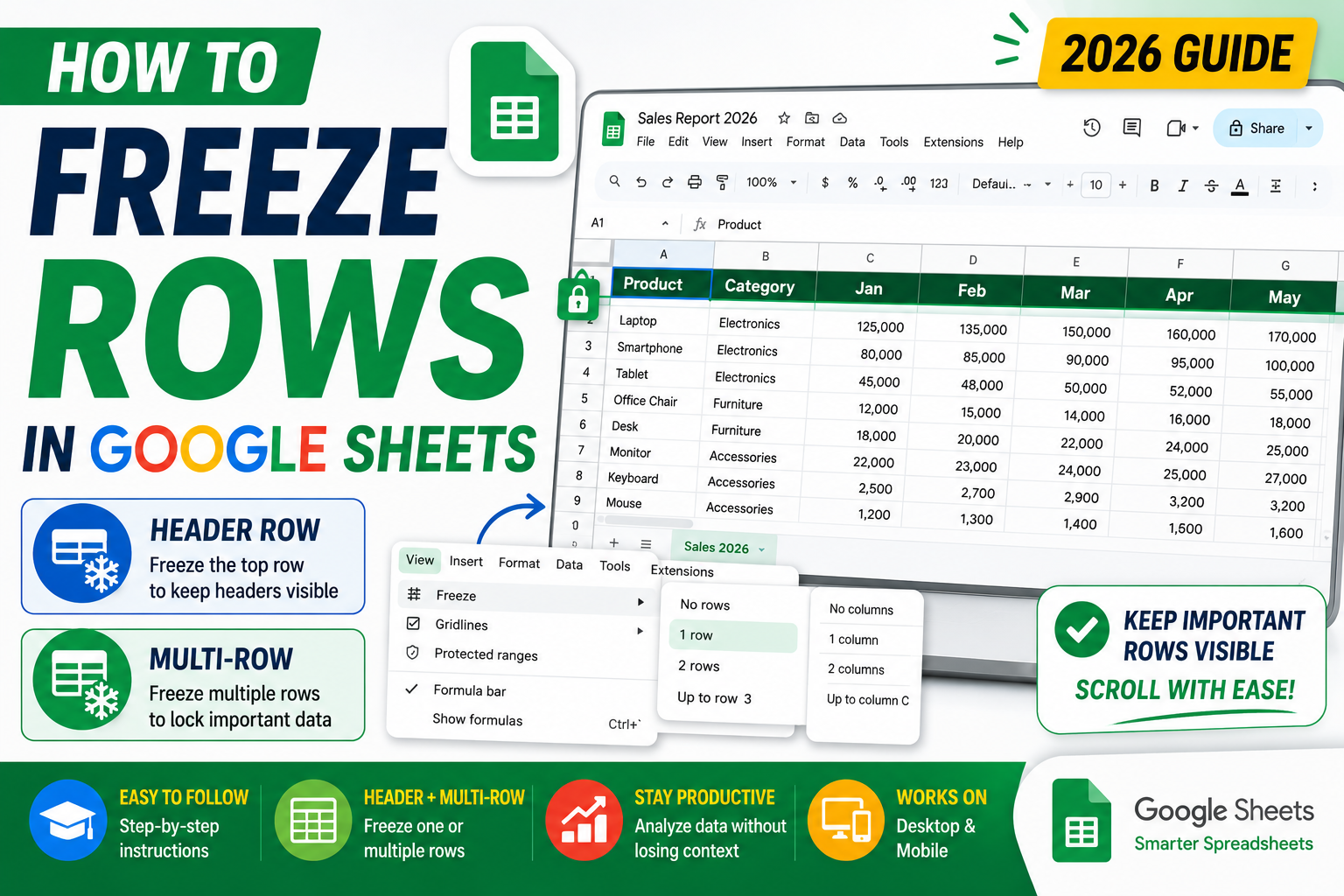
Quick step-by-step summary (click to expand)
- Open your Google Sheet. Go to sheets.google.com and open your file.
- Click View menu. Top menu bar.
- Hover over Freeze. A submenu opens.
- Pick your freeze option. 1 row, 2 rows, or up to current row.
- Verify the freeze. Scroll down. The frozen rows stay visible at the top.
- Adjust as needed. Drag the gray freeze bar up or down to change the freeze row count.
- Unfreeze if needed. View > Freeze > No rows.
Freeze the header row (most common)
The typical use case: your first row is a header (Column names like Name, Date, Amount). You want it visible always.
- Open your Google Sheet.
- Click the “View” menu at the top.
- Hover over “Freeze”.
- Click “1 row”.
A thin gray line appears below row 1. Scroll down and row 1 stays visible at the top.
Freeze multiple rows (2, 3, or custom)
Sometimes you have multiple header rows (title in row 1, subtitle in row 2, column names in row 3):
- Click “View” > “Freeze”.
- Choose “2 rows” to freeze the first two rows.
- For 3 or more: click the specific row number (or select a cell in that row), then choose “Up to current row” or “Up to row N” from the Freeze submenu.
Alternative drag method:
- Look for the thick gray bar at the very top of the column headers (just below the row 1 boundary).
- Click and drag that bar downward.
- Release when it sits below the row you want to be the last frozen row.
The drag method is faster once you know where the bar is (it’s tiny by default). Hover carefully to find it.
Freeze columns as well as rows
You can freeze both rows AND columns at the same time. For example, freeze row 1 (headers) AND column A (row labels):
- View > Freeze > “1 row”.
- View > Freeze > “1 column”.
Now scrolling in either direction keeps your headers/labels visible. Combined freeze is essential for wide spreadsheets with hundreds of columns.
Freeze rows on Google Sheets mobile
The mobile app has a slightly different flow:
- Open the Google Sheets app.
- Open your spreadsheet.
- Tap the row number of the LAST row you want frozen (e.g., row 2 to freeze rows 1 and 2).
- Tap the three-dot menu at the top right.
- Tap “Freeze”.
To freeze columns on mobile, tap the column letter instead of the row number, then follow the same menu path.
Unfreeze rows
To remove the freeze completely:
- Click View > Freeze > “No rows”.
- The gray line disappears. All rows scroll freely.
To reduce the number of frozen rows (e.g., from 3 down to 1), just pick “1 row” instead of “No rows”. The freeze count updates.
Freezing vs hiding: which to use when
- Freeze rows: Keep specific rows visible while you scroll. Rows are still active and part of formulas.
- Hide rows: Remove rows from view entirely. Rows are still there but not visible. Right-click a row number > Hide row.
- Filter rows: Show only rows matching your criteria. Data > Create a filter, then use column filters. Non-matching rows are hidden but data stays.
Freezing is for headers you want to always see. Hiding is for rows you rarely need. Filtering is for temporarily narrowing your view.
Freeze rows across multiple sheets in one workbook
The freeze setting is per-sheet, not per-workbook. Each tab of your Google Sheets file can have its own freeze setting. To apply consistent frozen headers across all tabs:
- Set the freeze on the first sheet.
- Switch to the second sheet.
- Set the same freeze.
- Repeat for each sheet.
There is no “apply to all sheets” shortcut. If you have many tabs, use a Google Apps Script to loop through and set the same freeze on each.
Common issues
- Freeze bar is invisible. It’s a very thin dark gray line just below the frozen row. Look carefully at the boundary between the last frozen row and the first scrolling row. Zoom in to 125% if you cannot see it.
- Frozen rows still scroll off screen. Refresh the browser tab. Occasionally Google Sheets does not apply the freeze on old sessions.
- Cannot freeze on mobile. Update the Sheets app. Older versions had a bug where freeze was hidden behind a longer menu path.
- Freeze disappears when I share the sheet. The freeze is preserved for collaborators, but if they have zoomed differently they may not see it correctly. Ask them to reset zoom to 100%.
- Print preview shows frozen rows repeating on every page. That’s the intended behavior for printing. If you don’t want it, unfreeze before printing or use File > Print > Formatting > “Repeat frozen rows” toggle.
Related: split view (alternative to freeze)
Google Sheets doesn’t have a native “split view” like Excel does. If you need to see two non-adjacent parts of your sheet simultaneously, workarounds:
- Open the same spreadsheet in two browser windows (right-click the tab > Duplicate).
- Use Data > Create a filter to focus on specific rows in one view.
- Use a helper column with a formula that references the row you want to keep tracking.
Freezing is the closest Sheets gets to split view.
Official documentation
Frequently asked questions
How many rows can I freeze in Google Sheets?
Practically unlimited but limited by the visible screen area. Frozen rows must fit above the scrolling area. In practice, most useful cases freeze 1 to 5 rows. Beyond 10 rows, you lose too much scrollable space.
Does freezing rows affect formulas?
No. Freezing is a visual setting only. Formulas, sorting, filtering, and data operations all treat frozen rows the same as any other row. It’s purely how the rows display on screen.
Can I freeze rows in the middle of a sheet, not just at the top?
No. Google Sheets only supports freezing rows from row 1 downward and columns from column A rightward. You cannot freeze rows 50-52 while letting 1-49 scroll away. If you need mid-sheet freezing, split the data into two sheets or use a helper filter view.
Does the freeze setting stay when I export to Excel?
Yes. When you download Google Sheets as .xlsx, the freeze setting transfers. Opening in Excel shows the same frozen panes. This makes freeze useful for shared workbook workflows where some collaborators use Excel.
Why does the freeze look different for different collaborators?
The freeze position is stored per-sheet globally, but browser zoom level affects visual layout. If a collaborator has zoomed in or out, the frozen rows may appear larger or smaller. Ask them to reset zoom to 100% (Ctrl+0) for consistent view.
Is there a keyboard shortcut to freeze rows?
Not directly. There is no built-in shortcut for View > Freeze. You can create one via a Google Apps Script bound to your account, but for one-off freezing, the menu path is fast enough (View > F > 1 row using arrow keys).