
In this tutorial, we will explain ISNA Excel function and how it handles #N/A errors. Along with other functions such as MATCH, IF and Vlookup we will determine how this ISNA function works with them.
Particularly, #N/A errors return when Excel cannot find the values looking for. The reason Excel provides ISNA function is to intercept and handle this error.
So, how it is significant it should be? Well, this function makes the formula more user-friendly and has a pleasant-looking worksheet.
What is ISNA function in Excel?
Excel ISNA function is a built-in handling function. Primarily, check formulas and cells #N/A errors and belongs to the category of Information functions.
Simply, this function is a way to identify if the given datasets, formula, or function contains #N/A error or not. Hence, it makes it more efficient to compare and for data analysis, thus accordingly fixing errors.
Further, this ISNA function can collaborate with other functions which are relevant such as IF or VLOOKUP wherein it will cover as we go on this topic. Meanwhile, it helps to perform extra operations based on the data sets in the worksheets.
Syntax
=ISNA(value)
Argument
value – This argument is a value to check if #N/A error.
Return Value
This returns logical values either TRUE or FALSE.
- TRUE: It will return TRUE only when #N/A error exists, based on the given parameter.
- FALSE: It will return FALSE if #N/A error is not existing in the given parameter. If this happens, you may create values to contain the parameter or error types.
Let’s see how this parameter works in the given data and formula in our table below.
| Data | Formula | Returns | Description |
|---|---|---|---|
| #N/A | =ISNA(#N/A) | TRUE | The ISNA function returns TRUE since the data given is #N/A error. |
| #NAME? | =ISNA(#NAME?) | FALSE | It returns FALSE since the value given is not #N/A error. |
| #DIV/0! | =ISNA(#DIV/0!) | FALSE | It still returns false even though the return value is error because it is not #N/A error. |
| Text | =ISNA(Text) | FALSE | The same way with TEXT values ISNA does not recognize it and return FALSE. |
How to use ISNA in Excel
Using ISNA excel function is usually used with the other function in evaluating the result of a particular formula. To start we will use it basic with its pure form first to understand it clearly.
Apparently, we only need to put a formula in the value argument of ISNA.
ISNA(your_formula())
And now we will try this in our worksheet, so in our sample data below we will compare column C and E. Wherein we will determine which product decreased sales.
In comparing the list of products in cell C3 against the list of products in column E, the formula is as follows:
=MATCH(B3, $E$3:$E$4, 0)
When the lookup value is found, using the MATCH function returns the value in the lookup relative position, otherwise it will output #N/A error. To check this result using the ISNA, we nested the formula.
Try the formula given below:
=ISNA(MATCH(B3, $E$3:$E$4, 0))
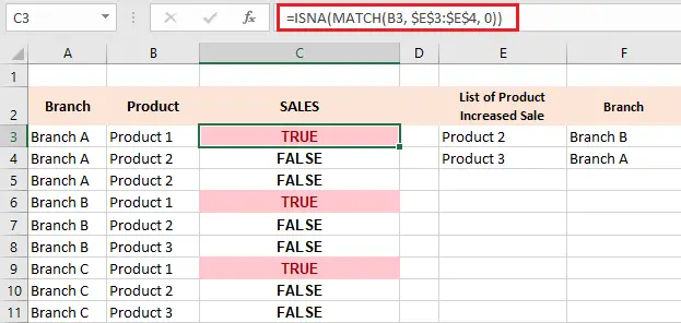
Afterward, just copy the formula on the rest of the rows from C3 to C11, or double-click the green plus sign to drag and copy the formula.
And now you see clearly which product decreased its sales — ISNA returns TRUE value– and the rest are products got increased its sales — ISNA returns FALSE value —.
IF ESNA Excel
Specifically, ISNA function only returns logical values TRUE or FALSE. However, if you want to display return a customized message, we will utilize this with the IF function.
IF(ISNA(…), "text_if_error", "text_if_no_error")
Examining our datasets example above, let’s identify which product increases its sales, thus return value “Increased SALES” while if the product decreased its sales it will return value of “Decreased SALES”.
Obviously, to make this happen we will embed ISNA and MATCH functions with IF logical test function. And now we created this formula:
=IF(ISNA(MATCH(B3,$E$3:$E$4,0)), "Decreased SALES", "Increased Sales")
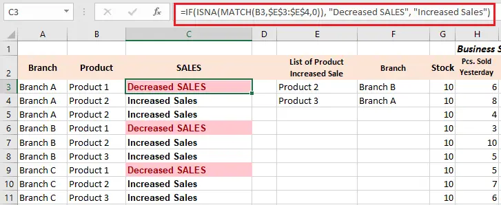
The result is now more readable and intuitive, right?
Hence, let’s explore a little further using this ISNA function along with Vlookup.
Excel ISNA Vlookup
The Vlookup in excel is one of the popular built-in functions which is usually used to extract data from a set of lists from another list. Apparently, the #N/A error is very common output of the Vlookup function.
Usually, this occurs when the function couldn’t find the lookup value in a given dataset.
Therefore to avoid displaying #N/A error which is inevitable to happen, it is better to display some meaningful error message or leave a blank space. This will makes the worksheet effective and professional.
Thus, ISNA became a useful one regarding this situation. When ISNA is utilized together with this function it supports determining the #N/A error based on the given data set.
Apart from that, we can nest the combined formula of ISNA and VLOOKUP functions within the IF function to return or retrieve a customized message in place of the #N/A error.
The syntax of ISNA function and Vlookup is shown below:
=IF(ISNA(VLOOKUP(…),"custom_message", VLOOKUP(…))
The custom message argument of the syntax is returned when the #N/A error exists in the dataset, otherwise Vlookup value result will be the return value.
In our example of dataset, we are going to display the branches of the product which increase its sales. Subsequently, it will display a return message “All Branches Decrease Sale” for the product decrease its sales in all branches.
Preferably, we need to create the basic VLOOKUP formula, the syntax is as follows:
=VLOOKUP (lookup_value, table_array, col_index_num, [range_lookup])
- lookup_value: It is a value to lookup.
- table_array: a range where the lookup value exists.
- col_index_num: It is a column number where the range of value must retrieve.
- range_lookup: It is the way we want to lookup. Use True or 1 for approximate match and FALSE or 0 for exact match.
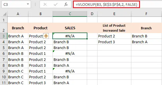
So, we lookup the what branch increased sales and which is not, below is the VLOOKUP formula:
=VLOOKUP(B3, $F$3:$F$4, 1, FALSE)
Then we combined the Vlookup formula in IF and ISNA formula we used in the above example. Take a look on the formula below:
=IF(ISNA(VLOOKUP(B3, $E$3:$F$4,2, FALSE)), "All Branches Decrease Sale", VLOOKUP(B3, $E$3:$F$4, 2, FALSE))
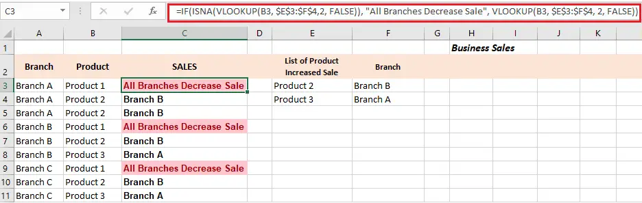
So we input this formula in cell C3 which we can copy into the rest of the rows.
Conclusion
In conclusion, this article about ISNA function is essential in making our worksheet more effective and professional wherein it allows replacing #N/A error in presenting the data.
However, it is important to keep in mind that ISNA function in Excel is not helping to locate the area where the #N/A area is present. Rather, it is a great help to inform you that there is an #N/A error in the specific field.
I hope you had learned a lot on this topic. Thank you for reading 🙂