
What is a pivot table?
A pivot table allows you to arrange data in various ways with just a few clicks.
It automatically analyzes, summarizes, sorts, and filters a huge amount of data.
In addition to that, it calculates the total and average of the data and presents the results in a reasonable manner.
Also, it has built-in percentage calculations available so that users can easily get the difference and compare data from different perspectives.
Calculating the percentage Difference in Excel Pivot Table
To calculate the percent difference in the pivot table, here are the steps you must follow:
Alternatively, if you don’t know how to use a pivot table, we’ve got your back.
1. Create a Pivot Table
- Open your Pivot Table in Excel and identify the two values you want to compare.
- Select the cell where you want to display the percentage difference.
- Click on the “Value Field Settings” option in the “Values” section of the Pivot Table.
- In the “Value Field Settings” dialog box, select the “Show Values As” tab.
- From the drop-down menu, select “% Difference From” and choose the base field and base item.
- Click OK to apply the changes.
After that here’s the next step:
- Select any cells in your current worksheet.
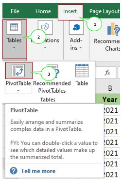
- Go to “Insert tab” in the menu bar or ribbon.
- Click “Tables,” and it will show the list of tables.
- Select “From Pivot Table/Range.” A dialog box will pop up.
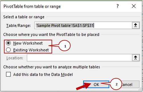
- In the “PivotTable from or range,” dialog box you can select the range that you want to use and choose where you want to put your pivot table, either in a new worksheet or an existing worksheet.
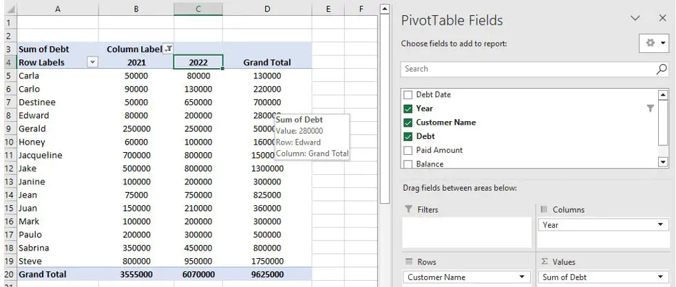
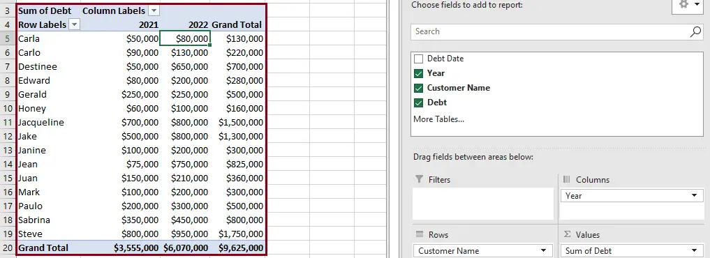
- In our case, we chose “New Worksheet,” and this is the result. You will see the PivotTable and PivotTable Fields.
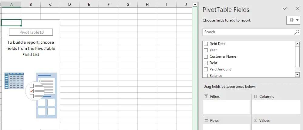
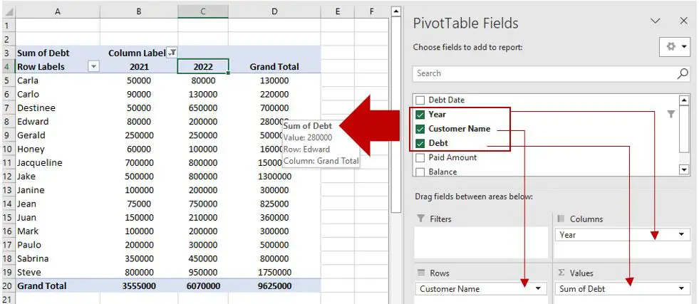
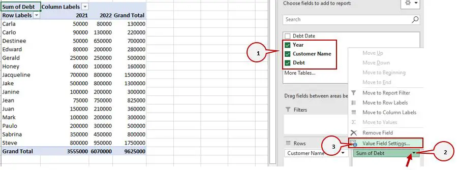
- Now, let’s add data to your pivot table. You may just check the data or drag it down to the drag fields area.
2. Calculate the percentage in the pivot table
After we added the data, it’s time to calculate the percentage in the pivot table.
To see the percent difference between the year 2021 and 2022, here’s the thing that you should follow:
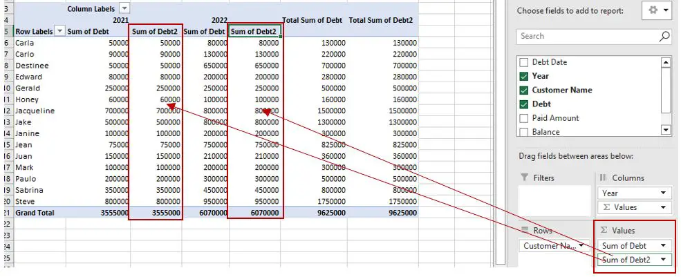
- Add another unit value to the values area, where it will become “Sum of Debt 2.”
- Drag the “Debt” to the “Values”
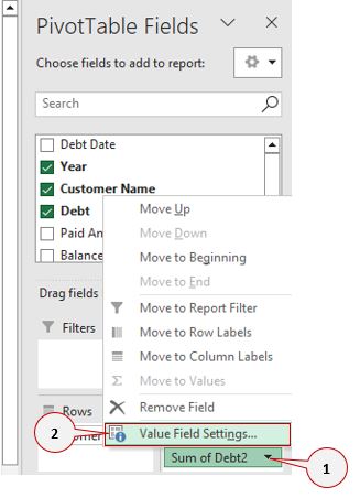
- Click the drop-down arrow of “Sum of Debt 2.”
- A context menu will pop-up and select “Value Field Settings.”
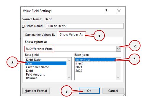
- In the “Value Field Setting” dialog box, select “Show Values As.”
- Then, click the drop-down list for “Show values as” and choose “% Difference From.”
- Under “Base field,” select “Year” because that is what we wanted to see the difference between years “2021-2022.”
- On the right side under “Base item,” select “(previous)” and then click “OK.”
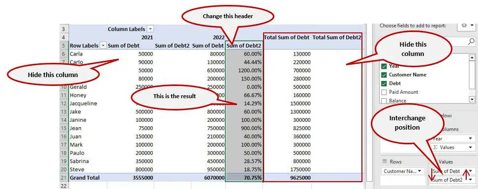
This is the outcome after you click the “OK” button. We just need to flourish something to make it more professional.
First, we need to remove or hide columns that are no longer needed, and second, we need to change the header of “Sum of Debt 2” into “% of Difference.”
Lastly, we need to interchange the positions of sum of debt and sum of debt 2.
Now, take a look at the final result of the percentage difference in the Excel pivot table.
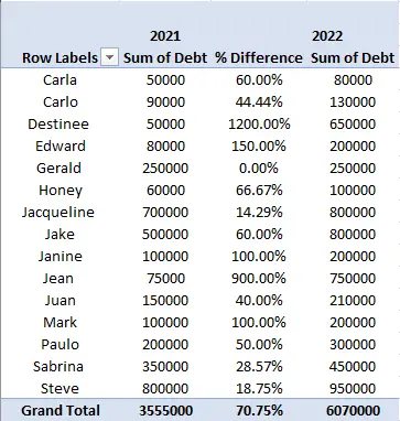
The image shows that the debt increased during 2022, and as you can see, it is easy to understand the difference between 2021 and 2022 using the percentage difference in an Excel pivot table.
Another way to calculate percentage difference in Excel
This way of calculating the percentage difference is the same as how to create a pivot table in the above steps; however, their distinction is the process of calculating.
So we are going to show you a step-by-step tutorial on calculating the percentage difference in this way.
We are using same sets of data.
- Check or drag the data to the drag fields.
- Click the drop-down arrow for “Sum of Debt.”
- It will pop up a context menu, then select “Value Field Settings.”
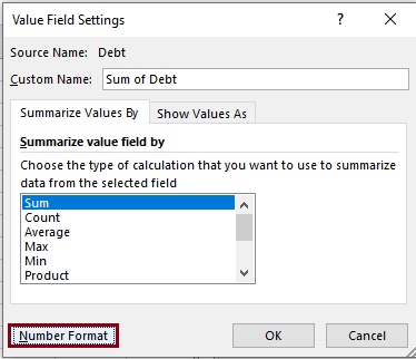
- In the “Value Field Settings” click “Number Format,” and it will display “Format Cells” dialog box.
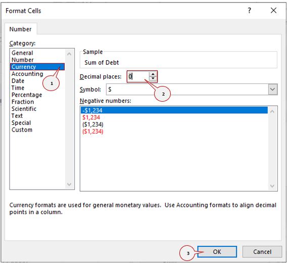
- In the “Format Cells” dialog box, select “Currency.”
- Choose “0” in the “Decimal places” box.
- Then, click the “OK” button and also the “OK” button in “Value Field Setting.”
Result:
We are almost there; you just need to follow these steps to calculate and get the difference.
In this section, we will use the “Fields, Items, & Sets” option to calculate the percentage difference between the columns 2021 and 2022.
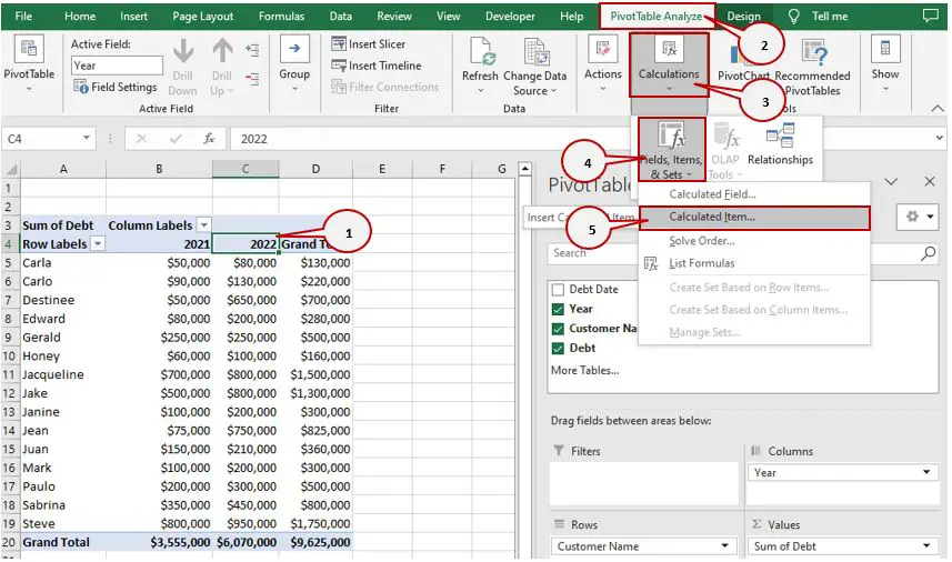
- Click the cell for either the years 2021 or 2022.
- Select “PivotTable Analyze” in the ribbon or menu bar.
- Click “Calculations,” and it will show a context menu.
- Then, select “Calculated Item,” and it will show a dialog box.
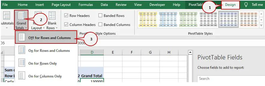
Note: Hide the grand total because we are not going to use it anymore.
Now, it’s time to calculate and add another field that will contain the percentage difference between of 2021 and 2022.
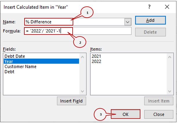
- In the Insert Calculated Field wizard, input “% Difference” in the “Name” field or whatever name you want to put.
- In the formula, you can double-click the data under “Items,” or you can just input the formula.
Note: The formula is "=2022/2021-1."
- Then after that click the “Ok” button.
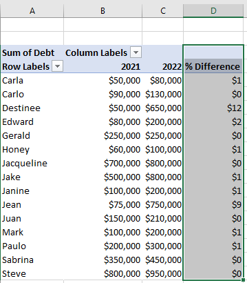
Finally, we already added a new column that contains the results, but we need to change the number format.
We are not yet finished; we are going to change the result to percent. After that you’ll get the following result.
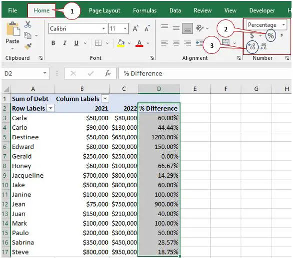
- Go to the “Home” tab.
- Select the percent icon “%.”
- Click twice the left decimal places icon, and the data in the pivot table will automatically change.
- When you’re done, you can customize your pivot table based on your requirements.
At last, we get the calculated percentage differences between the debt years 2021 and 2022.
How to analyze the Percentage difference in Excel pivot table
After you’ve done calculating the percentage difference in the Excel pivot table, here are the following pieces of information you may use to make data-driven decisions:
- Identify the patterns and trends in your data.
- Compare the results for different periods of years or products.
- Evaluate the percentage results of your data.
- Keep track of the changes of your data.
Tips and Tricks
- You must understand the procedure on how to do it to avoid continuous error.
- Focus on the data that you want to compare and see the difference between two sets of data.
- You may customize your pivot table by adding filters, rows, and columns in order to focus on the important data.
- Formatting Pivot Table makes it more visually appealing and certainly it is easy to understand.
- Add conditional formatting to highlight cells that contain low and high percentage differences.
- For instance, create graphs and charts; by doing so, it is easy to visualize your data and identify trends.
Conclusion
This article covers the step-by-step guide that calculates the percentage difference in a pivot table.
By following this guide, you can easily calculate percentages in Excel using a pivot table.
Just don’t forget to customize your pivot table and use charts and graphs to visualize your data.
We are hoping that you will find this tutorial useful, and we would love to hear some thoughts from you.
If you found this tutorial to be a valuable resource, please leave a comment below.
Thank you very much for continuing to read until the end of this article. In case you have more questions or inquiries, feel free to comment below.

Caren Bautista
Technical Writer at PIES IT Solution
Responsible for crafting clear, well-structured, and beginner-friendly content across the platform. Handles the writing, proofreading, and editorial review of tutorials, guides, and documentation to ensure every article is accurate, readable, and easy to follow.
Expertise: Technical Writing · Content Creation · Documentation · Editorial Writing · JavaScript · TypeScript · Python · Python Errors · HTTP Errors · MS Excel · View all posts by Caren Bautista →