What is a Pivot Table?
A pivot table is an essential Excel feature that helps users quickly organize and summarize complex data.
This feature allows users to group their data by columns, sort it by values, and calculate statistics.
In addition, pivot tables are handy when you have a large quantity of data. Before proceeding to our tutorial, first learn how to create a pivot table.
How to Create a Pivot Table
If you want to create a pivot table, you should have your data set. Once you have your data, you can start creating pivot tables.
Here’s a tutorial on how to make one:
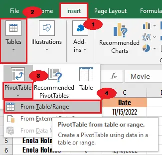
→ Click anywhere on your data, then the Insert tab. In the Tables group, click PivotTable, then select “from table/range.”
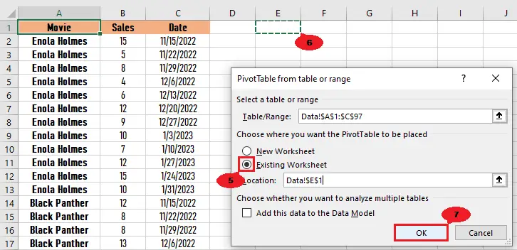
→ After clicking “from table or range,” a PivotTable from table or range dialog box will appear.
Select “new worksheet” if you want to place your pivot table on a new worksheet.
However, select “existing worksheet” if you want to place your pivot table on the same worksheet as your data, then select a cell where you want to place it and click OK.
Formatting a Pivot Table in Excel
The following are simple steps to format a pivot table in Excel.
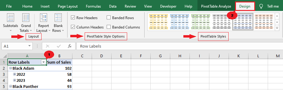
- Click anywhere in the pivot table.
- Click the design tab under PivotTable Tools.
After clicking the design tab, you’ll see three groups. The Layout group, the PivotTable Style Options group, and the PivotTable Styles group.
Tip: You can also right-click the pivot table, then select format cells. After that, a format cells dialog box will appear. Then, you'll see number, alignment, font, border, fill, and protection tabs (see image below).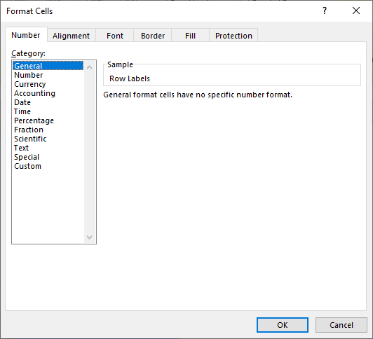
Change the Pivot Table Styles
To change the style of a pivot table, click the More button in the PivotTable Styles group.
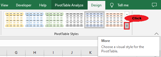
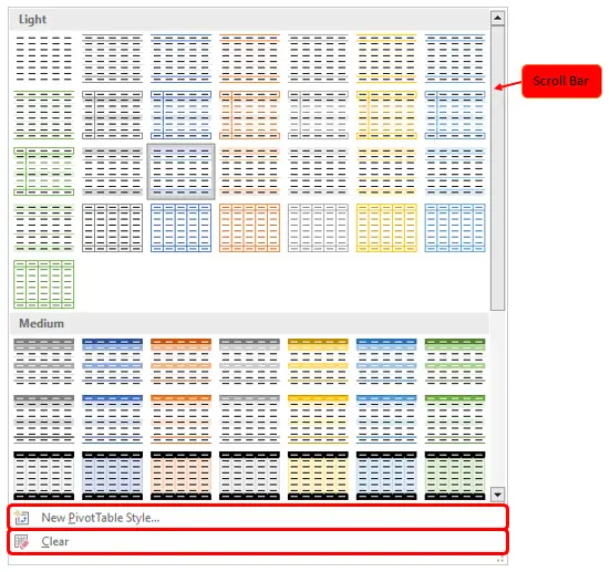
After clicking the “more” button, you’ll see the PivotTable styles gallery.
There, you can choose the style that you want for your pivot table.
- You can scroll down the scroll bar to see more designs.
- You can also click the new PivotTable Style to create a new PivotTable Style.
- And you can also click Clear to clear the table style.
PivotTable Style Options
In the pivot table style options, you’ll see:
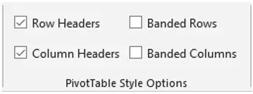
- Row Headers, which can show special formatting for the first row of the table.
- Column Headers, can show special formatting for the first column of the table.
- Banded Rows, which format even rows differently from odd rows.
- Banded Columns, which format even columns differently from odd columns.
You can check or uncheck any of these four based on your preferred format.
Format the Pivot Table Layout
In the Layout group, you can format the following:
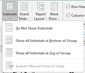
- Subtotals. Here, you can show or hide subtotals of your data.
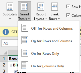
- Grand Totals. Here, you can show or hide the grand totals of your data.
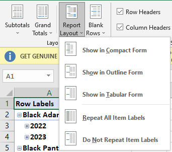
- Report Layout. Here, you can adjust the report layout.
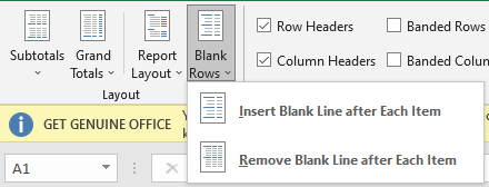
- Blank Rows. Here, you can insert and remove blank lines after each item.
Conclusion
In conclusion, formatting a pivot table in Excel is easy and quick. Learning how to do it is also an easy thing to do. Just follow the simple steps in the tutorial above.
I believe that we have accomplished this tutorial. I hope you’ve learned something from this. Do not forget to share this with your friends.
If you have any questions or suggestions, please leave a comment below, and for more educational content, visit our website.
Thank you for reading!

Elijah Galero
Programmer & Technical Writer at PIES IT Solution
Elijah Galero is a programmer and writer at PIES IT Solution, author of 175+ tutorials at itsourcecode.com. Specializes in Python error debugging (AttributeError, TypeError, ModuleNotFoundError), Python programming tutorials, and Microsoft Excel how-to guides for BSIT students and productivity learners.
Expertise: Python · Python Errors · Python AttributeError · Python TypeError · ModuleNotFoundError · MS Excel · MS PowerPoint · View all posts by Elijah Galero →