
In this tutorial, we will explain what is Excel Subtotal function and how to use it in manipulating the worksheet.
Subtotal function in Excel
The subtotal function is designed to return the subtotal in a list or database. This calculates the range of cells and ignores cells that should not be included. Unlike other functions which are created for single purposes only, subtotal is amazingly versatile.
So here are the following features which make subtotal special:
- It ignores automatically filtered out-of-view rows.
- In the same manner, ignores existing subtotal formulas to avoid double counting.
- It can execute different arithmetic and logical functions such as Sum, Average, Count, IF, Min and Max.
The good thing about this function is it’s available in all versions of excel such as Excel 2016, Excel 2013, Excel 2010, Excel 2007, and lower.
Moving let’s familiarize the syntax of this function. So that we can able to create a formula based on this function.
Syntax
=SUBTOTAL(function_num, ref1, [ref2],…)
Return Value
A number representing its specific kind of subtotal.
Arguments
- function_num – it is a number which specifies the function to be used in the calculation of subtotals within the list.
- ref1 – It is the range or reference to be subtotal.
- ref2 -An optional argument, still the range or reference to subtotal.
Further, the function_num argument can be one of the following lists:
- 1 – 11 does ignore filtered-out cells but includes manually hidden rows.
- 101 – 111 does ignore all hidden cells – filtered out and hidden manually.
| Include hidden | Ignore hidden | Function | Description |
|---|---|---|---|
| 1 | 101 | AVERAGE | Function presents the average of numbers. |
| 2 | 102 | COUNT | Counts cells that have numeric values. |
| 3 | 103 | COUNTA | Counts non-empty cells. |
| 4 | 104 | MAX | Finds the largest value. |
| 5 | 105 | MIN | Finds the smallest value. |
| 6 | 106 | PRODUCT | Computes the product of cells. |
| 7 | 107 | STDEV | Returns the standard deviation of a population based on a sample of numbers. |
| 8 | 108 | STDEVP | Returns the standard deviation based on an entire population of numbers. |
| 9 | 109 | SUM | Add all the numbers. |
| 10 | 110 | VAR | Estimates the variance of a population based on a sample of numbers. |
| 11 | 111 | VARP | Estimates the variance of a population based on an entire population of numbers. |
Actually, you don’t need to memorize the list above, because when you enter subtotal formula it displays the list of functions including their number. It’s easy for you right?
For instance, this is how can you create a Subtotal 9 formula to sum up the values in cells G3 to G10:
How to use Subtotal function in Excel
Time needed: 2 minutes
Here are the simple steps which will guide you to use subtotal function in your worksheet.
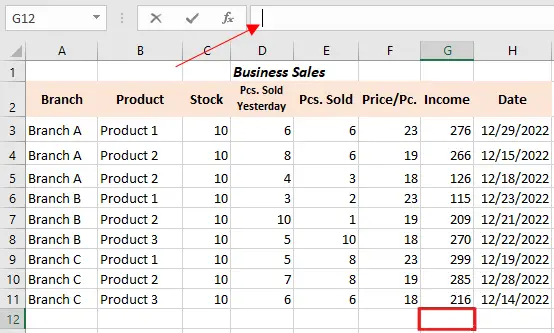
- Select Empty Cell
Upon opening Excel worksheet, make sure it contains data. Select empty cells where you want output to return.
Once you select, click the formula bar and assure the blinking cursor is active.
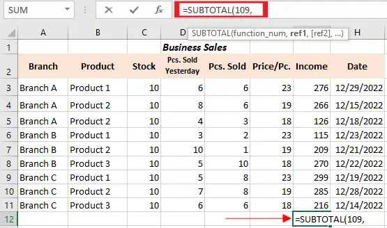
- Insert the function_num method
As you begin to create a subtotal formula, type =SUBTOTAL( — in formula bar or selected cell.
The first argument of SUBTOTAL formula is function_num which is relevant to another mathematical function. So, just type a number from 1 to 11 which means it includes hidden values either 101 to 111 to ignore them.
For our example, =SUBTOTAL(109, this will use SUM function which will add the range of cells and exclude all hidden values. Nonetheless, you can select methods automatically as the options menu will display under the formula.
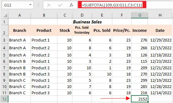
- Select Subtotal ranges
At the next stage, you’ll need to specify the required ref2 cell range. This is the data that the SUBTOTAL formula will use to calculate a subtotal.
And now, it’s time to select the subtotal ranges. This requires specifying ref2 cell range. Moreover, this is the data to be utilized in subtotal calculation. If you want to add multiple ranges you can insert this one for another.
In our case, we sum the ranges of cells G3:G10 and C3:11.
Here is the formula we created: =SUBTOTAL(109, G3:11, C3:C11)
Remember always close the formula with a parenthesis.
Note: If the range of data is invalid Excel will return error. To fix this you must remove or change the conflicting data utilized in SUBTOTAL.
Excel Subtotal Common Error
If you encounter error in using Excel Subtotal in your worksheet data, the following might be a reason:
#VALUE! — this happens when function_num argument is not from integer 1-11 or 101-111 or only ref arguments contain 3-D arguments
#DIV/0! – This error happens when a specific summary function is required to execute a division by zero.
#NAME? – the SUBTOTAL function is misspelled.
How to insert Subtotals using the SUM function in Excel
Microsoft Excel Subtotal has known to have 2 sets of number functions: 1-11 and 101 -111. These are sets that ignore filtered-out rows. However, the number 1-11 includes manually hidden rows thus 101-111 exclude them.
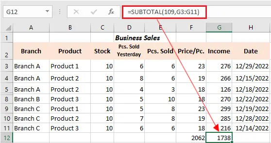
To know the total sum of filtered rows, use either Subtotal 9 or Subtotal 109 displayed in the image below:
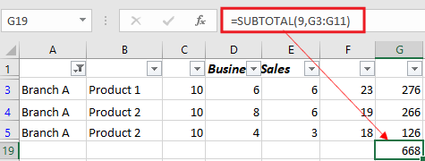
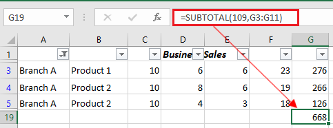
But if we have manually hidden irrelevant data using the Hide rows command. So on the Home tab > Cells> Group> Format> Hide & Unhide, or by just simply right-click the rows then click hide.
Hence, we will total values that only have visible rows and the number function we should is the Subtotal 109 option.

Conclusion
In conclusion, Excel Subtotal function is quite helpful in analyzing data quickly, without being dependent to pivotable.
However, if you are having a hard time with subtotal, you can also use another possible way which is the Subtotal feature in Data Tab of the ribbon bar.
Thank you for reading 🙂

Glay Eliver
Programmer & Technical Writer at PIES IT Solution
Glay Eliver is a programmer and writer at PIES IT Solution, author of over 600 tutorials at itsourcecode.com. Specializes in JavaScript tutorials, Microsoft Office how-tos (Excel, Word, PowerPoint), and Python error debugging covering ImportError, TypeError, AttributeError, ModuleNotFoundError, and JavaScript ReferenceError. Authored several of the site’s highest-traffic Excel and MS Office reference articles.
Expertise: JavaScript · MS Excel · MS Word · MS PowerPoint · Python · Python ImportError · Python TypeError · Python AttributeError · ModuleNotFoundError · JavaScript ReferenceError · Pygame · View all posts by Glay Eliver →