How to Calculate Weighted Average in Excel Pivot Table

In this guide, we will show you how to calculate the weighted average in an Excel pivot table.

For example, we have a set of data with a pivot table. We wanted to calculate its weighted average.

Here’s the complete guide on how to do it:

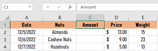
1. Add a helper column to the source of data.

   
   Since Excel doesn’t have a feature in the pivot table that automatically calculates the weighted averages, we add a helper column and name it Amount.
   
   Note: Insert the column within or inside your data set, not after your last column. If you just input new data next to the last column of your data set, it will not be included in your pivot table once you already have one, even if you refresh it.
   
   

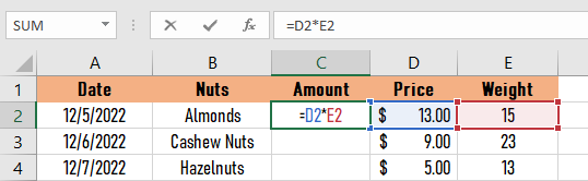
2. Type =C2*D2.

   
   After creating a helper column, type the formula =C2*D2 in the first cell of the helper column, which is your amount column.
   
   

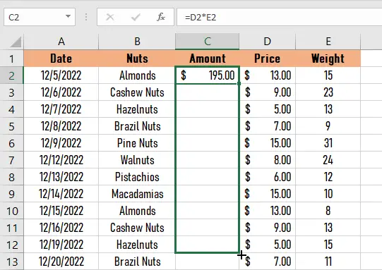
3. Drag the autofill handle to fill all the columns.

   
   To automatically fill all the columns with the given formula, drag the autofill handle until the last row of your data.
   
   
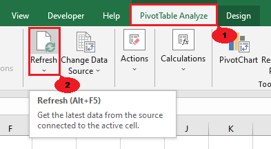
4. Select anywhere in your pivot table, then click PivotTable Analyze > Refresh.

   
   After the third step, go to your pivot table. Select any cell in it, then click PivotTable Analyze under the PivotTable Tools, then click Refresh.
   
   

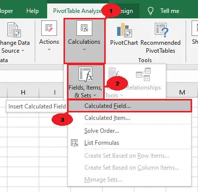
5. Select Calculations > Field, Items, & Sets, then click Calculated Field.

   
   Once your pivot table is refreshed, go to the Calculations group, select Fields, Items, & Sets, then click Calculated Field.
   
   

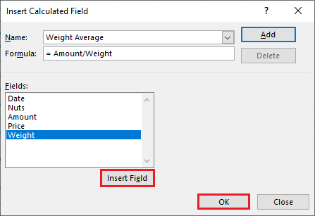
6. Edit the Insert Calculated Field Dialog Box.

   
   After clicking the Calculated Field button, an Insert Calculated dialog box will appear. Here are the steps for what you’re going to do next:
   
   1. Rename the text in the name’s textbox into Weight Average.
   2. Insert the field Amount, input the “/” symbol, then insert the Weight field in the formula textbox.
   3. Click OK.
   
   
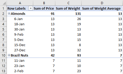
7. Result.