
It is important to know the different shortcuts for filtering data in Excel when working with huge amounts of data.
Excel is an invaluable tool when it comes to data analysis, sorting, categorizing, and a lot more.
How to filter Excel data quickly using keyboard shortcuts?
Using keyboard shortcuts, we can make the process faster and, of course, more efficient. We will now discover the different keyboard shortcuts for filtering data.
Use this shortcut:
1. You just press and hold the “Alt” key, then press the “D” key, followed by the “F” key twice (“Alt + D + F + F”).
This will activate the “Filter” command and that will allow you to filter your data in Excel.
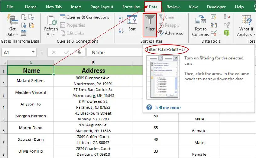
2. “Ctrl + Shift + L” is another shortcut to filter data in an Excel spreadsheet.
3. Press CTRL + T to bring up the Create Table dialog box, and then press Enter to create your table.
Refer to the video below.
You can see below the different shortcuts to filter in Excel.
1. Turning filters on or off in Excel
1. Select any cell, or if you have a data range that contains any blank columns or rows, you need to select the entire cell in your data range that you want to filter.
2. Click the “Data” tab in the menu bar.
3. Then, click the “Filter” option in the “Sort & Filter” section. You can also use Ctrl+Shift+L to add and remove the filter.
4. After you click “filter,” filter dropdowns will appear in the header of your data, as you can see in the image below.
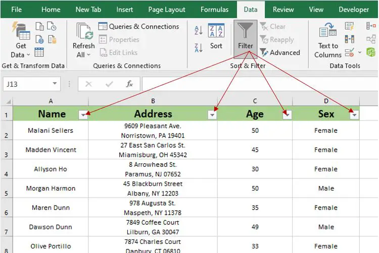
5. You can now sort your data based on your requirements.
Note: You can turn on and off the filter by pressing Ctrl+Shift+L.
2. Showing the Dropdown Filter Menu in Excel
1. Select the cell in your header row, and it should have a filter drop-down icon.

2. To open the filter menu, press ALT + then the down arrow key on the keyboard.
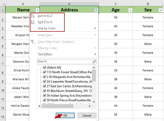
3. At this point, you can sort from A to Z or Z to A, depending on your requirements.
Note: The keyboard shortcut to open the drop-down menu is Alt+Down Arrow.
3. Keyboard Shortcuts for the Filtering Drop-Down Menus in Excel
1. You must first press Ctrl+Shift+L to show the drop-down filter in your header row.
2. To access the drop-down menu, press Alt+Down Arrow.
Below are the full keyboard shortcuts for the filter drop-down menu:
Alt+Down Arrow+S -Sort A to Z.
Alt+Down Arrow+O -Sort Z to A.
Alt+Down Arrow+T -Sort by Color submenu.
Alt+Down Arrow+I -Filter by Color submenu.
Alt+Down Arrow+F -Text Filters.
4. Selecting menu items using arrow keys
If the Filter menu is being displayed, you can use the arrows to navigate the menu, Enter, and the Spacebar to select and apply filtering:
Press the up or down arrow keys to select a command.
Press Enter to apply the command.
Press the Spacebar to check or uncheck the checkbox.
Note: Make sure that the drop-down filter is enabled for the keyboard shortcuts (arrows, enter, and spacebar).
Conclusion
This tutorial about the “Different Shortcuts To Filter In Excel Like A Pro“ would be a great help for everyone.
Hence, using these keyboard shortcuts to filter your data in Excel can save you a significant amount of time and effort.
By mastering these shortcuts, you will be able to filter your data quickly, and apart from that, it will be easy for you to analyze and interpret the data.
Thank you very much for continuing to read until the end of this article. In case you have more questions, feel free to comment below.

Caren Bautista
Technical Writer at PIES IT Solution
Responsible for crafting clear, well-structured, and beginner-friendly content across the platform. Handles the writing, proofreading, and editorial review of tutorials, guides, and documentation to ensure every article is accurate, readable, and easy to follow.
Expertise: Technical Writing · Content Creation · Documentation · Editorial Writing · JavaScript · TypeScript · Python · Python Errors · HTTP Errors · MS Excel · View all posts by Caren Bautista →