
What is a pivot table in Excel?
A pivot table in Excel allows you to arrange data in various ways with just a few clicks. It automatically analyzes, summarizes, sorts, and filters a huge amount of data.
As well as it calculates the total and average of the data and presents the results in a reasonable manner.
Apart from that, users can easily compare data from different perspectives.
Why use a Pivot Table?
A pivot table in Excel provides various advantages for data analysis, such as:
- It simplifies a complex set of data.
- Sort and visualize huge amounts of data in a user-friendly way.
- It summarizes the data by categories and subcategories.
- It creates custom reports and improves efficiency in data analysis.
- Pivoting enables you to rotate rows and columns to visualize different summaries of the presented data.
- It presents the subtotal and aggregate numerical data in your worksheet.
- The level of data expands, collapses, and digs down to see the details behind any total.
- Output concise and engaging online data or printed reports.
Keyboard shortcuts for creating a pivot table in Excel
Creating a pivot table in Excel is a simple process that can be accomplished in just a few clicks.
1. Basic steps in creating a pivot table in Excel
Here are the basic steps:
- Select any cells in your current worksheet.
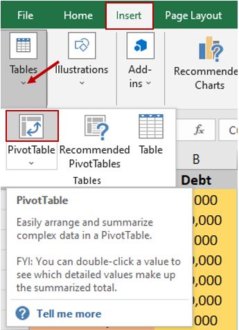
- Go to the “Insert tab” in the menu bar.
- Click “Tables,” and it will show the list of tables.
- Select “From Pivot Table/Range.” A dialog box will pop up.
- In the “PivotTable from or range,” dialog box you can select the range that you want to use.
- And, choose where you want to put your pivot table, either in a new worksheet or an existing one.
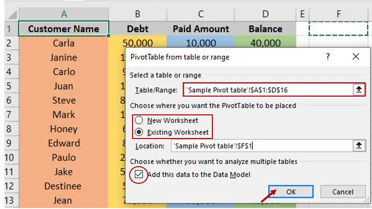
Note: Don’t forget to check the “Add this data to the Data Model” if you want analyze multiple tables.
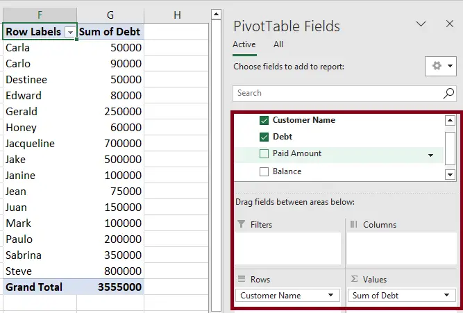
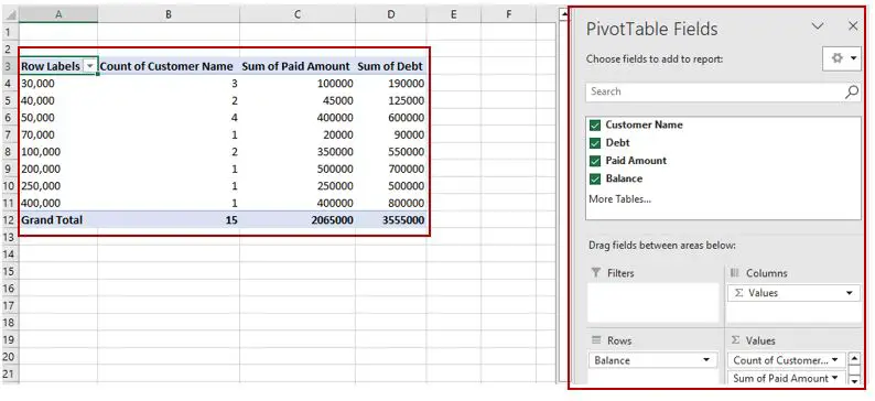
- Check the data to show in the pivot table layout or drag and drop the fields PivotTable Fields pane.
However, we found the two recommended shortcut methods to easily create and open a pivot table in Excel quickly and efficiently:
2. Recommended PivotTable Option
Using the Recommended PivotTables option allows you to create a pivot table in Excel with just a few clicks. Here’s the following step on how to use it:
- Select any cells in your worksheet or the entire range of your data.
- Click “Insert” and select “Tables.”
- Then, choose the “Recommended PivotTables” option.
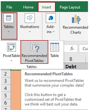
- Excel will provide you with the recommended pivot table, which you may use; it just depends on your requirements.
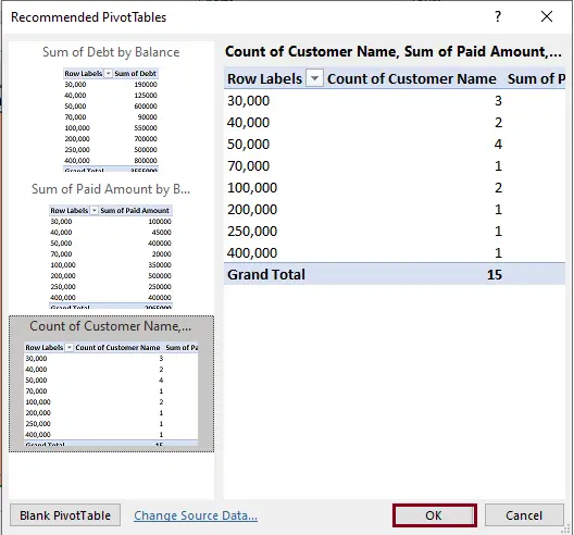
- This is the result.
3. Keyboard Shortcut to create a pivot table in Excel
Using the keyboard shortcuts allows you to create pivot tables in Excel quickly and easily.
Here are the following steps on how to use it:
1. Alt + D + P is the shortcut key to open the pivot table in Excel
- Select any cells or the entire data set that you want to analyze.
- Press the “Alt” + “D” + “P” keys on your keyboard.
- After that, it will pop up the pivot table wizard. Kindly refer to the video below:
List of keyboard shortcuts for pivot table
The keyboard shortcuts for pivot tables are invaluable and definitely helpful when you are using pivot tables in Excel.
It would be fun to learn new things, especially in Excel, where it is convenient for you and helps to speed up your work.
Here is the list of pivot table keyboard shortcuts:
| PivotTable Shortcut | Function |
|---|---|
| ALT + D + P | To open pivot table wizard |
| ALT + N + V | Used to create a pivot table |
| Ctrl + A | To Select the entire pivot table |
| F11 | Used to insert pivot chart to a new Sheet |
| ALT + F1 | Used to add a pivot chart to the current worksheet |
| Spacebar | Toggle checkboxes in pivot table fields list |
| ALT + Shift + Left Arrow Key | To ungroup selected pivot table items |
| ALT + Shift + Right Arrow Key | To Group selected pivot table items |
| ALT + JT +L | Used to view or hide field list |
| Ctrl + (-) Minus | Hide item from the pivot table |
| Alt + F5. | Refresh the current pivot table |
| Ctrl + Alt + F5. | Refresh all pivot tables in the workbook |
Aside from that, we also have a list of Excel shortcut cheat sheets for more advanced keyboard shortcuts that you may use.
Conclusion
With this tutorial on a shortcut to a pivot table in Excel, you can obtain relevant insights. These insights can speed up your work and improve your data analysis.
These various shortcuts for pivot tables in Excel will definitely help and save you time and effort.
They can be accomplished using the keyboard or the basic option that you discovered above.
We would love to hear some thoughts from you. If you found this tutorial to be a valuable resource, please leave a comment below.
Thank you very much for continuing to read until the end of this article.

Caren Bautista
Technical Writer at PIES IT Solution
Responsible for crafting clear, well-structured, and beginner-friendly content across the platform. Handles the writing, proofreading, and editorial review of tutorials, guides, and documentation to ensure every article is accurate, readable, and easy to follow.
Expertise: Technical Writing · Content Creation · Documentation · Editorial Writing · JavaScript · TypeScript · Python · Python Errors · HTTP Errors · MS Excel · View all posts by Caren Bautista →