
What is Distinct Count in Excel Pivot Table?
A distinct count in Excel pivot tables is one of the powerful tools in Excel that allows you to count and determine the number of unique values in a given data set.
In addition to that, it has always been equal to or less than count.
The count is different from distinct because the count is the total number of values, and it counts the duplicate values.
However, distinct count is the total of different values or the number of unique values, and it doesn’t include duplicate values.
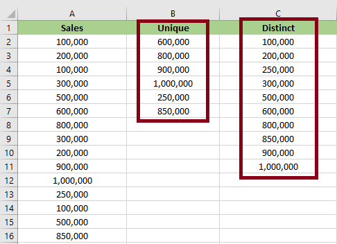
What is the Difference between Unique Count and Distinct Count?
| Unique values | Distinct values |
|---|---|
| Unique count is the total number of values that occur only once in the data set. | Distinct count is the total number of different values nevertheless it occurs many times still it is counted as one distinct count. |
In a very brief statement, values that are repeats or duplicates are not unique. Whereas distinct are those values that appear at once, even if the value appears multiple times, it is still counted as one.
Let’s take a look at our example below:
As you can see in the image, you can easily determine the difference between the two data sets.
Note: Unique and distinct count are not thesame.
How to use and get distinct counts in an Excel pivot table
This time, we will explore how to get unique and distinct values in Excel using formulas, and we’ll also show you how to use distinct counts in an Excel pivot table.
Adding a Distinct Count in Excel using Pivot Table
Using a data model is the best and easiest way to get a distinct count in Excel. Follow the following guide:
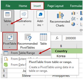
- Click the cell that contains your data, and then click “Insert” in the menu bar.
- Click “Tables,” and it will show the list of tables.
- Select “From Pivot Table/Range.” It will show a dialog box.
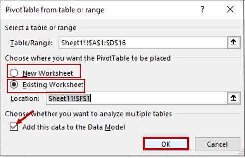
- In “PivotTable from or range,” dialog box you can choose where you want to put your pivot table, either in a new worksheet or an existing worksheet. In our case, we chose “Existing Worksheet.”
- When you choose “Existing Worksheet,” you have to click any cell where you want to display your pivot table in your current worksheet, and then it will display in the “Location.”
- But if you choose “New Worksheet,” it will open a new worksheet.
- Don’t forget to check the checkbox “Add this data to the Data Model.”
- Then click “OK.”
9. It will look like this after you click “OK.”
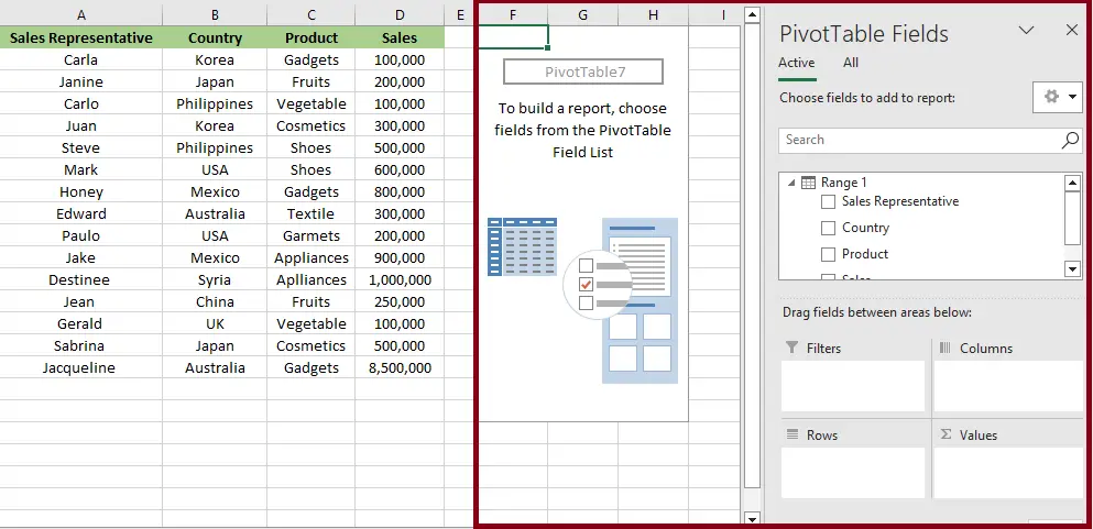
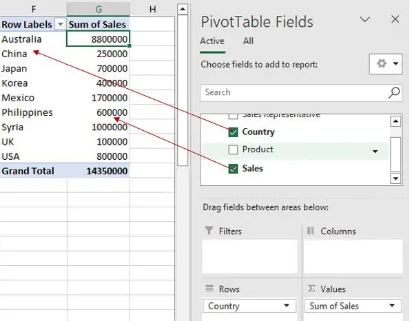
10. Now it’s time to get a distinct count, but first we have to add data to your pivot table layout.
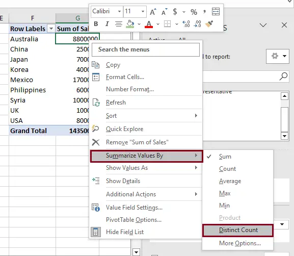
11. Right-click the value of “Sum of Sales” in our case, then click “Summarize Values By” and choose “Distinct Count.”
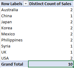
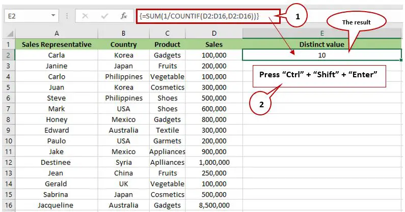
12. As a result, you’ll get a 10 distinct count for sales in the pivot table.
Kindly check the video below; it contains a step-by-step guide from the beginning and different ways on to get a distinct count in the Excel pivot table.
Note: For those who are using Excel 2013, 2016, 2019, and Microsoft 365, the only thing you do is access the data model.
Adding a Distinct Count in Excel using the Function
To get the distinct count without using a pivot table in Excel, you just need the formula in order to get the distinct values.
Especially when you are holding huge amounts of data, we know that it’s hard to do it manually.
We need to use this formula: = SUM(1/COUNTIF(range, range)). Why do we use COUNTIF? It is because we need to find out how many times each value appears on your worksheet, particularly within the specific range.
Take a look at our example below:
Note: Don't put a bracket sign in your formula bar; it only appears due to the shortcut key that we use, "Ctrl" + "Shift" + "Enter," in order to get the exact value.
Formula to get a distinct count in Excel
1. =SUM(IF(1/COUNTIF(data, data)=1,1,0))
Note: You have to press the "Ctrl" + "Shift" + "Enter" shortcut rather than the usual Enter keystroke, because it is an array formula.
2. =SUMPRODUCT(1/COUNTIF(range, range))
Tip: if you want the usual keystrokes, you may use the formula above.
Counting Distinct numbers using a Formula
Use ISNUMBER to get the distinct count values (time, date, and number) in Excel.
Here’s the formula: =SUM(IF(ISNUMBER(range) or = 1/COUNTIF(range, range),””)).
Here’s the thing that you should do:
- Click the cell where you want to put the data. Then, input the formula in the formula bar.
- Right after you create the formula, don’t press Enter right away.
- Press “Ctrl” + “Shift” + “Enter” to get the exact value.
Counting Unique and Distinct Counts in Excel
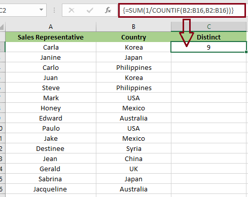
In our example below, we want to get the unique value of a country using a formula, and we get a value of 3 and a distinct value of 9.
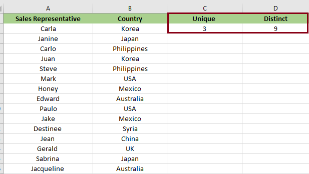
The formula to get the Unique value is =SUM(IF(COUNTIFS(B2:B16,B2:B16)=1,1,0)). Whereas the formula we use in the example is =SUM(1/COUNTIF(B2:B16,B2:B16)).
Conclusion
This simple tutorial on how to get the distinct count in an Excel pivot table will be able to help you get the value of distinct in a large amount of data.
We also provided a formula to get the unique and distinct values in all versions of Excel if you don’t want to use a pivot table.
With the help of this guide, you will be able to differentiate between unique and distinct values.
Thank you very much for continuing to read until the end of this article. In case you have more questions, feel free to comment below.

Caren Bautista
Technical Writer at PIES IT Solution
Responsible for crafting clear, well-structured, and beginner-friendly content across the platform. Handles the writing, proofreading, and editorial review of tutorials, guides, and documentation to ensure every article is accurate, readable, and easy to follow.
Expertise: Technical Writing · Content Creation · Documentation · Editorial Writing · JavaScript · TypeScript · Python · Python Errors · HTTP Errors · MS Excel · View all posts by Caren Bautista →