How to Edit Pivot Table in Excel: A Step-by-Step Tutorial

Pivot Table in Excel

A pivot table in Excel allows you to arrange data in various ways with just a few clicks. It automatically analyzes, summarizes, sorts, and filters a huge amount of data.

As well as it calculates the total and average of the data and presents the results in a reasonable manner.

Apart from that, users can easily compare data from different perspectives.

How to add or insert a pivot table in Excel

Here are the things that you need to follow when adding a pivot table in Excel. You have to organize your data first.

Arrange it in tabular format with a header. It will be easier for you to select your data when adding a pivot table.

1. Select any cells in your current worksheet.
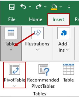
2. Go to “Insert tab” in the menu bar.
3. Click “Tables,” and it will show the list of tables.
4. Select “From Pivot Table/Range.” A dialog box will pop up.
5. In “PivotTable from or range,” dialog box you can select the range that you want to use and choose where you want to put your pivot table, either in a new worksheet or an existing worksheet.

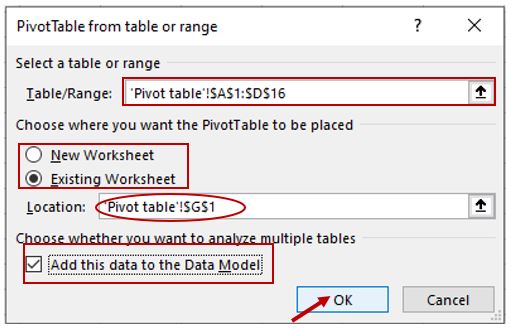
7. When you choose “Existing Worksheet,” you have to click any cell where you want to display your pivot table in your current worksheet, and then it will display in the “Location.”
8. But if you choose “New Worksheet,” it will open a new worksheet.
9. Don’t forget to check the checkbox “Add this data to the Data Model.”
10. Then click “OK.”

This is the result:

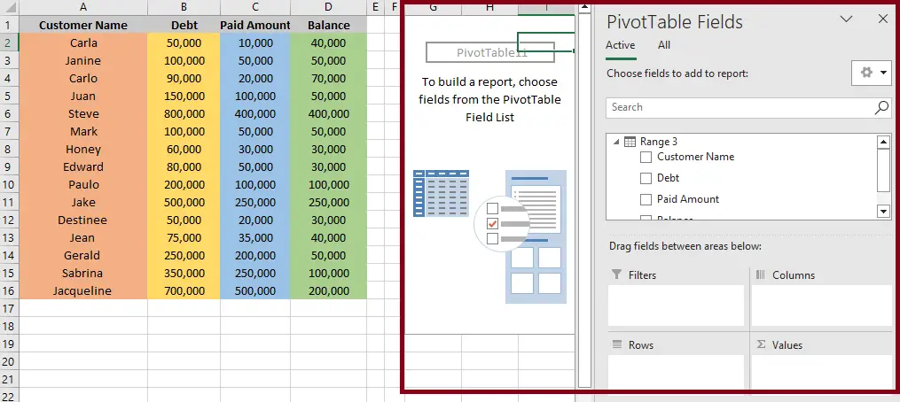
Finally, you’re done inserting your pivot table, and now it’s time to add data and edit your pivot table.

Kindly refer to the video below:

How to edit pivot tables in Excel

Now, let’s explore what you should do when updating pivot tables in Excel.

After you added the pivot table to your worksheet, you may now start to edit it.

You can add or delete fields, change the calculation type, and change the data format.

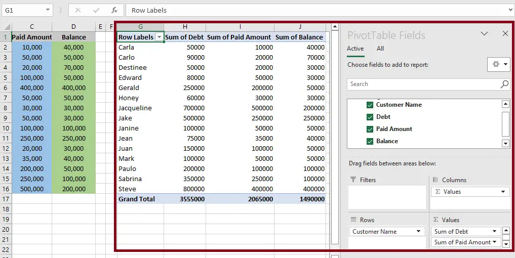
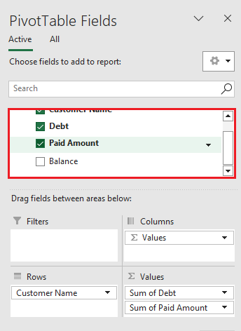
To add a field

1. Check the fields under “Choose fields to add to the report.“
2. Or else, simply drag the data in “Drag fields between areas below:” from the Field List to the Rows or Columns area.

To remove or delete a field

1. Click on the drop-down arrow next to the field name and select “Remove Field.”

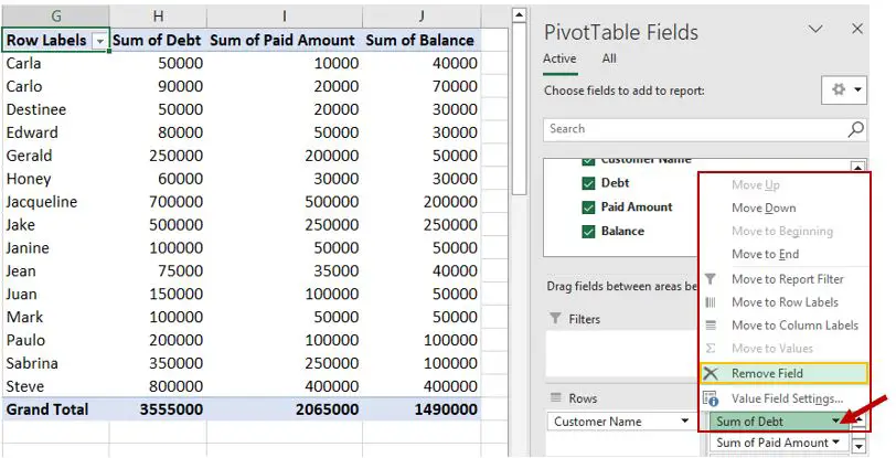
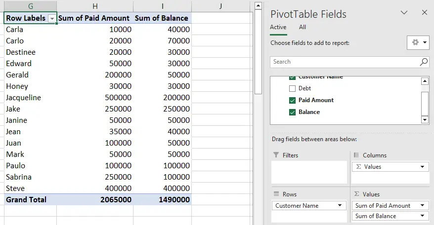
Result: The sum of debt has been successfully removed from your pivot table.

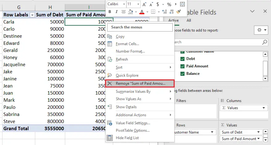
Or you can do:

1. Right-click the data, and a context menu will display.
2.  Select “Remove.” It will automatically remove the data.

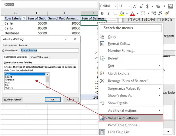
To change the calculation or value type

You can also right-click the data and choose “Value Field Settings.”

Another way to change the value type.

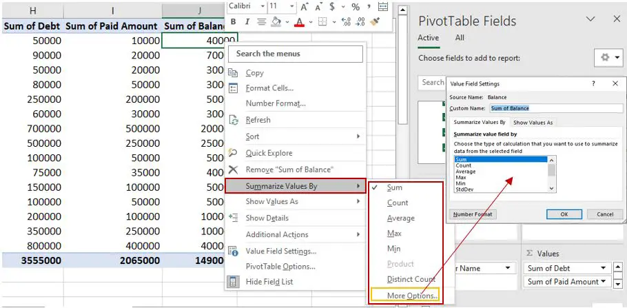
1. Right-click the data that you want to change its calculation type.
2. After you right-click, a context menu will pop up.
3. Select “Summarize Values By,” and it will display different value types.
4. If you want more value types, just click “More Options.” A “Value Field Settings” dialog box will display.
5. Then, click the “OK” button. It will automatically change the value of your selected row of data. Refer to the image below.

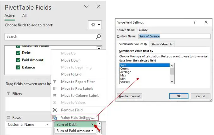
1. Click on the drop-down arrow at the right side of the field name and select Value Field Settings.
2. A “Value Field Settings” dialog box will pop up, and you can choose what value type you want.
3. Click the “OK” button. Refer to the image below.

Note: Don’t forget to refresh if you make changes to your data so that tour pivot table will update.

If you make changes to your data, you will need to refresh your pivot table in order to update it.

To do this, just click on the Analyze tab and then click on the Refresh button. This will automatically update the pivot table.

Change Pivot Table Data Source

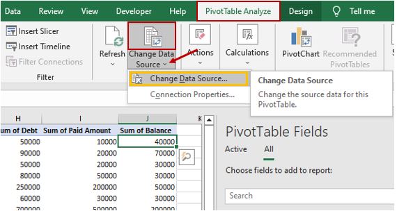
1. Click “Analyze,” which in our case is “PivotTable Analyze” because of our worksheet name.
2. Select the “Change Data Source” icon or drop-down arrow to select “Change Data Source.”

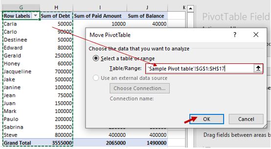
3. A “Move PivotTable” and then in the “Table/Range:” You can choose a range of cells and add another piece of data, either in your current cell or in another worksheet.
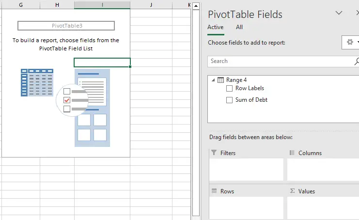
4. It will show, like in the image below, that you select data by just checking it or by dragging it to the “Drag fields between areas below:”

Conclusion

This step-by-step tutorial on how to edit a pivot table in Excel will help users easily create, remove, and edit their pivot table in less than a minute.

Users will definitely save time and increase their efficiency when working by using this guide.

Thank you very much for continuing to read until the end of this article. In case you have more questions, feel free to comment below.

What is new when editing PivotTables in 2026

The 2026 Excel channel update renamed the Analyze tab on the ribbon to PivotTable Analyze to prevent confusion with the general Analyze Data (Copilot) feature. All buttons stayed in the same positions, so keyboard tips like Alt JT F for Field List still work.

Microsoft also added a Suggested changes button in the Copilot pane. Click any PivotTable and open Copilot, and the pane recommends edits such as swapping a row field for a column field or adding a running total. Accept a suggestion with one click, and Copilot writes the change into the PivotTable.

Common editing mistakes to avoid

• Editing labels in the PivotTable cells directly. Type-overs of Row or Column labels do not save. Rename the field in the Field List (right-click the field, choose Field Settings, edit Custom Name) instead.
• Deleting fields with Delete key. Pressing Delete on a PivotTable value clears the value but keeps the field slot. Drag the field OUT of the Values area to remove it cleanly.
• Editing after a refresh shifts positions. Manual sort orders and custom groupings can reset when the source has new categories. Lock the sort with More Sort Options > Sort Automatically each time the report is updated.
• Formulas referencing PivotTable cells. If a downstream formula uses GETPIVOTDATA, changing the PivotTable layout can break the formula. Disable Generate GetPivotData under PivotTable Analyze > Options if you need plain cell references.

Editing a Data Model PivotTable

A PivotTable connected to the Data Model (with Add this data to the Data Model checked at creation) uses DAX for calculated fields. Right-click any field and choose Add Measure to write a DAX formula, then use the measure as a Values field. Standard calculated fields (PivotTable Analyze > Fields, Items, Sets) are unavailable for Data Model PivotTables. Use measures instead.

Quick step-by-step summary (click to expand)

1. Click inside the PivotTable Click any cell inside the PivotTable to activate the PivotTable Analyze and Design tabs on the ribbon.
2. Add, remove, or rearrange fields Use the PivotTable Field List (right side) to drag fields between Rows, Columns, Values, and Filters, or uncheck fields to remove them.
3. Change how a value is calculated Right-click any Values field, pick Summarize Values By, and choose Sum, Count, Average, Max, Min, or Distinct Count.
4. Update the source data range Go to PivotTable Analyze, click Change Data Source, and select the new range. Click OK to apply.
5. Refresh to apply changes Press Alt F5 or click PivotTable Analyze > Refresh to pull the latest data from the source.