
In this tutorial, we will go over the Excel strikethrough shortcuts in greater detail with different methods. If you are working, taking shortcuts would save your time and effort and make your life easier.
How are you going to apply strikethrough in your Excel spreadsheet? Here, we will show you various methods or shortcut keys for strikethrough in Excel.
Let us now explore Excel strikethrough shortcuts in detail and apply them to your text.
What is Strikethrough?
A strikethrough is a font effect that is applied to text where a line appears. It runs through the center of the text as if it were crossed out. The text is marked as finished, removed, or mistaken.
It is called a character format, so it can be easily removed and applied in the text document. It is represented by a horizontal line.
Strikethrough is used for:
- Complete tasks.
- Suggest a revision.
- Imply humor.
- Indicates that the content is invalid or out of date
What is Strikethrough in Excel?
A “strikethrough” in Excel is a feature that creates a line through text. Most likely, it just means that the activity has been completed, which is why it has been checked off.
In addition to that, you can apply strikethrough to a cell or even a group of cells. The ribbon, the Format Cells dialog box, or a keyboard shortcut are all options.
Where is the font Strikethrough option?
1. Click the cells that you want to apply the strikethrough.
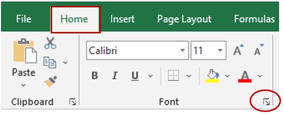
2. Click “Font Setting,” and then the Format Cells box will appear.
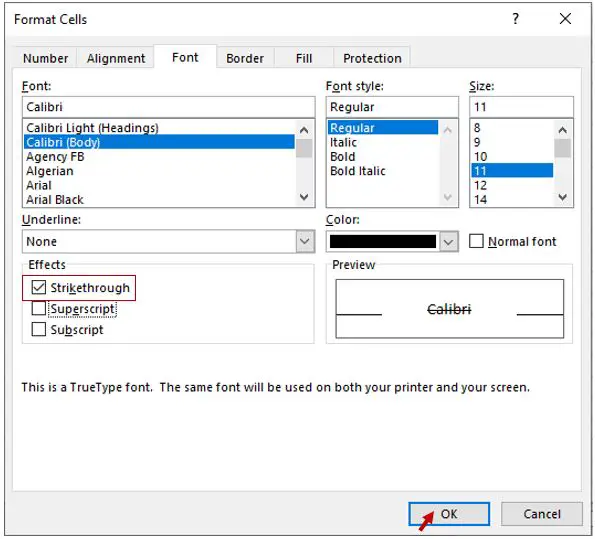
3. In the “Format Cells box,” check the strikethrough check box and click “OK.“
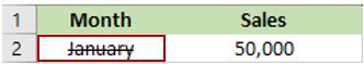
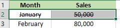
4. This is the outcome of your text when you apply strikethrough.
Different Ways to Apply Strikethrough in Excel
Let’s look at some different ways to apply strikethrough to text in an Excel spreadsheet.
1. Applying strikethrough using keyboard shortcut key
- Select the cell(s) to which you want to apply the strikethrough format.
- Then, press Ctrl+5. It will automatically apply it to your text.
- If you want to remove the strikethrough from your text, the same process will apply (press Ctrl+5).
You can also use Ctrl+Shift+F.
- 1. Choose a cell (or cells).
- 2. Press Ctrl + Shift + F.
- 3. Select strikethrough.
- 4. Click “OK.”
2. Applying strikethrough using the Format Cells dialog box
1. Click the cells that you want to apply the strikethrough.
2. Click “Font Setting,” and then the Format Cells box will appear.
3. In the “Format Cells box,” check the strikethrough check box and click “OK.“
4. This is the outcome of your text when you apply strikethrough.
3. Adding strikethrough using Quick Access Toolbar
First, we are going to add a strikethrough to your Quick Access Toolbar.
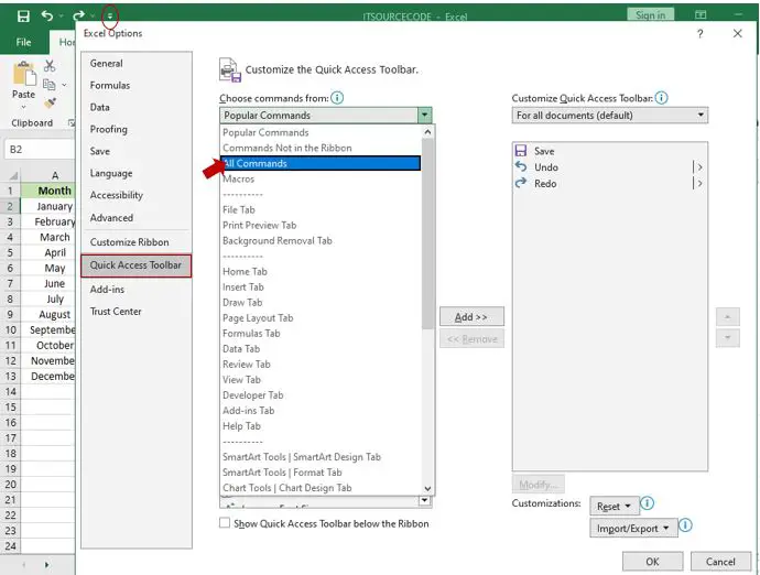
1. In the upper part of your Excel, click the arrow down beside the redo and undo icons. After that, in the “Choose command,” select “All Commands.”
2. After you click “All commands,” it will show a list. You just need to select strikethrough and click “Add >>” then click “OK.”
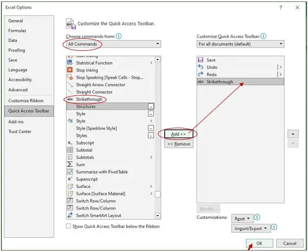
3. The strikethrough symbol has been successfully added to the Quick Access Toolbar.

4. Now you can easily add strikethrough to your text.
- a. Select the text to which you want to apply strikethrough.
- b. Click the strikethrough icon, and it automatically appears in your selected text.
4. Adding Strikethrough using Format Cells Option
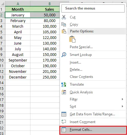
1. Choose the cell(s) to which you want to apply the strikethrough format. Then right-click and choose “Format Cells…”
2. In the “Format cell” dialog box, click “Font,” then check the checkbox for strikethrough, and click the button “OK.”
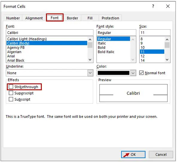
3. After you click the “OK” button, strikethrough is applied to your text.
5. Adding Strikethrough using it from Excel Ribbon
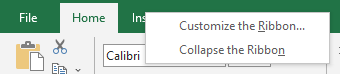
1. Right-click any tab in the menu bar and choose the “Customize the Ribbon” option.
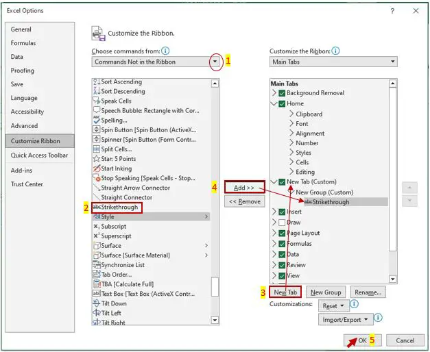
2. After you click “Customize the Ribbon,” “Excel Option dialog box will display. Under of “Choose commands from.”
- a. Click the drop-down list and choose “Commands Not in the Ribbon.”
- b. Select strikethrough.
- c. Select “New Tab,” a new Tab will appear in the “Main Tabs” section.
- d. When you click the “Add” button, a strikethrough appears under “New Group (Custom).”
- e. Lastly, click the “OK” button.
3. After that process, you’ve successfully added the strikethrough in the menu bar under “New Tab.”
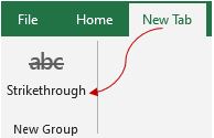
4.
Conclusion
I hope that all of the “Excel Strikethrough Shortcuts” mentioned above will be of great assistance to you and that you will use them in your Excel spreadsheets. The easiest way to speed up your work is to know about Excel shortcuts.
This article has already revealed the secret and simplest shortcut for adding strikethrough to your Excel spreadsheet, which is Ctrl + 5.
Thank you very much for continuing to read until the end of this article. In case you have more questions, feel free to comment. You can also visit our website for additional information

Caren Bautista
Technical Writer at PIES IT Solution
Responsible for crafting clear, well-structured, and beginner-friendly content across the platform. Handles the writing, proofreading, and editorial review of tutorials, guides, and documentation to ensure every article is accurate, readable, and easy to follow.
Expertise: Technical Writing · Content Creation · Documentation · Editorial Writing · JavaScript · TypeScript · Python · Python Errors · HTTP Errors · MS Excel · View all posts by Caren Bautista →