This tutorial will explain the XLOOKUP function of excel, which is a new lookup function for vertical and horizontal. Executing the last match, vlookup along with multiple criteria is now easier to accomplish as ABC.
Hence this replaces the VLOOKUP function, thus it is more versatile and flexible wherein we can use it in various situations.
Technically, this excel function can look up ranges from vertical to horizontal. The good thing is this function can perform an exact match, approximate and even wildcards(*?) in partial matches.
Moreover, it can do searching of data from its first value and last value, unlike other functions like VLOOKUP, HLOOKUP, LOOKUP.
XLOOKUP excel function syntax
The XLOOKUP formula as the name suggests searches range or specified value of array which returns the corresponding value from another column. The syntax of the function can search both horizontally and vertically wherein executing exact match, approximate, and wildcard.
Here is the syntax:
XLOOKUP(lookup_value, lookup_array, return_array, [if_not_found], [match_mode], [search_mode])
| ARGUMENTS | DESCRIPTION |
| Lookup_value | The value to look up for. |
| Lookup_array | The array or range where to search happens. |
| Return_array | The array or range that returns the value. |
| If_not_found (Optional) | The arguments return if the value is not found. Thus if forgotten returns #N/A error. |
| Match_mode (Optional) | This argument performs the match type: 0 or omitted (default) – The Exact Match. Returns #N/A if not found. -1 – exact match or next smaller. If the value is not found it returns the nearest smaller value. 1 – exact match or next larger. The next large value is returned if an exact match is not found. 2 – wildcard match. |
| Search_mode Argument (Optional) | It is the direction of search: -1 or omitted (default) – used to search from first to last -1 – look up a reverse order from last to first 2 – binary search on data relying on sorted in ascending order. -2 – binary search on data depending on sorted in descending order. |
How to Use Excel XLOOKUP Examples
Here are the following examples that will indicate how useful this function. As you explore the given examples, you will discover significant usefulness of Microsoft Excel.
Example 1: Basic Exact Match
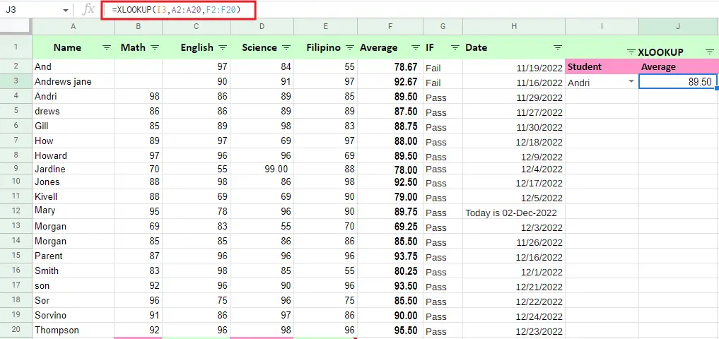
This function returns the exact match by default. In the given example, we use XLOOKUP to obtain an average based on the exact match of students. The formula is like this:
=XLOOKUP(I3,A2:A20,F2:F20)
Example 2: Basic Approximate Match
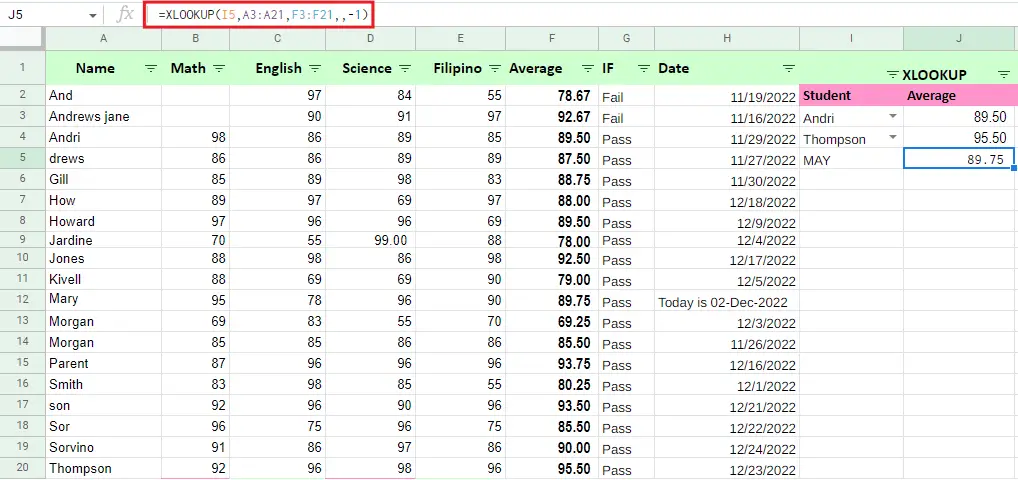
The best thing about this function it can provide a value for the match_mode argument. In the given example below, we are going to calculate the average of students named MAY which requires an approximate match. We supplied the formula -1 for match_mode. This will yield an approximate match or the next smallest.
The formula is given below:
=XLOOKUP(I5,A3:A21,F3:F21,,-1)
Example 3: Not Found Message
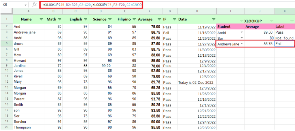
Basically, like other functions, if it can’t find the value it will return #N/A error. However, it will supply a value not_found to do this just enclose it in double quotes (“”). Take a look at this example below:
=XLOOKUP(J4,F2:F20, G2:G20,"Not found")
You can customize this message as you like: “No match”, “Movie not found”, etc
Example 4: Two-way Lookup
This function also allows nesting wherein it will perform a two-way lookup. In our example below the entire row will retrieve by the inner xlookup which will be handed to the outer as a return array.
=XLOOKUP(J5,B2:B20,G2:G20,XLOOKUP(J5,F2:F20,G2:G20))
XLOOKUP Multiple Criteria
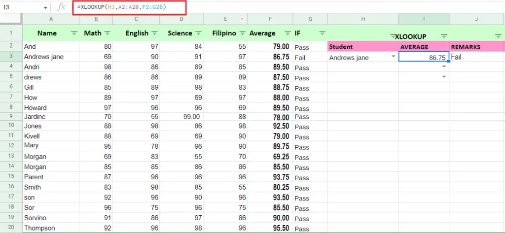
One of the advantages of XLOOKUP is to carry arrays which allow calculating multiple criteria using the direct lookup_array argument:
=XLOOKUP(H3,A2:A20,F2:G20)

XLOOKUP vs Vlookup
This time will know what’s better between XLOOKUP and VLOOKUP. As mentioned above, it is more advantageous than VLOOKUP. Now let’s find out in the following list:
- The XLOOKUP can look up both vertically and horizontally.
- Unlike VLOOKUP which searches only the left column, XLOOKUP has no limitations it can absolutely look up any directions.
- XLOOKUP returns an exact match by default, unlike VLOOKUP which returns an approximate match as default.
- Wildcards come in handy, unlike other lookups which require more work.
- If you’re skillfully fond of xlookup you can able to drag all the columns you need to return required values.
- It allows searching with multiple criteria
- Alternatively, you can customize your error message when the return value can not be found.
- It allows you to insert and delete columns without compromising the formula, unlike VLOOKUP which uses column index numbers wherein a bit hassle when some columns are removed.
- It is efficient wherein it only holds return arrays and lookup data. Meanwhile, VLOOKUP requires the entire table calculations, which need more cells.
XLOOKUP value error
This #VALUE! error happens when the lookup value and the return arrays are not compatible. For instance, the look-up horizontal array cannot return value from the vertical array.
Conclusion
To sum up, we learn from the article XLOOKUP Function Step-by-Step Guide With Examples:
- XLOOKUP can perform with both horizontal and vertical arrays.
- #N/A error means lookup value is not found.
- The lookup_array needs to have proportions which is compatible with the return_array argument nevertheless it will display #VALUE!
Thank you for reading!


