
In this tutorial we learn how to create pivot table in excel, thus we will learn what is pivot table and how to use it in working your data.
Having a large amount of data using pivot table is the quickest and most handy way to obtain an interactive summary of huge data.
What is Pivot Table?
Pivot table of excel is a powerful tool that summarizes an enormous amount of data. Apart from it allows you to utilize it in the quickest and easy way, a beginner in excel can readily use it. Its like you are dragging and dropping columns or rows in creating your report.
These are the characteristics and a pivot table capable to:
- Visualize large amounts of data in a user-friendly way.
- It summarizes data by categories and subcategories.
- Pivot table capable to filter, sort and conditionally formatting a set of data so that you can concentrate on the most relevant information.
- Pivoting enables to rotate rows and columns to visualize different summaries of the presented data.
- It presents the subtotal and aggregate numerical data in your worksheet.
- The level of data expands and collapses and digs down to see the details behind any total.
- Output concise and engaging online data or printed reports.
Components of Pivot Table
Before using pivot table and use it efficiently. Let us familiarize ourselves first with the components of pivot table.
- Pivot Cache — The snapshot of data excel takes and stores in its memory. This happens every time create a pivot table using the data.
- Values Area –it is the area that holds the calculations or values.
- Rows Area — It is the headings to the left of the Values area that make the Rows area.
- Columns Area — It is the headings at the top of the Values area that make the Columns area.
- Filters Area — is an optional filter that you can use to further drill down into the data set.
How to make Pivot Table
Here we will create pivot table, along with its steps and figures to make it simpler to understand.
- Enter your data into a range of rows and columns.
In this step, we need to prepare data that will be present in rows and columns in a spreadsheet. Basically a pivot table is from an Excel table. So if you don’t have ready worksheet, just input the value in specific rows and columns.
Additionally, the topmost row or column is the one that categorizes the values presented.
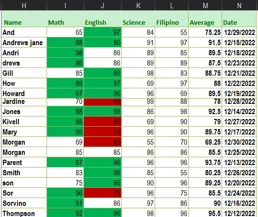
For example, we have the grades of the students. Let us see how it is presented.
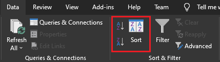
- Sort your data by preferred attribute.
This sort the data available to have easier access and manage when turning it into a pivot table. To this on the Data tab navigate to the Sort command.

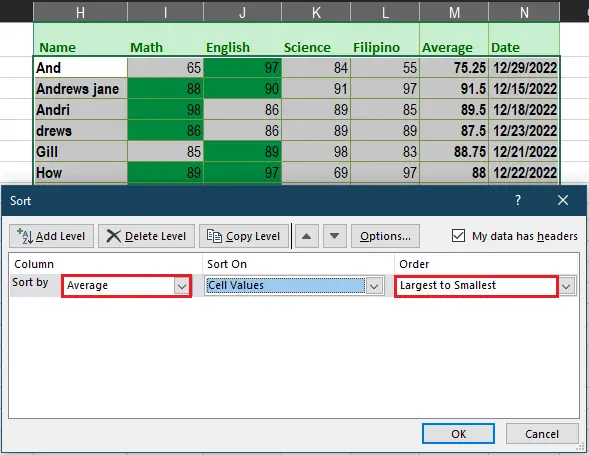
Along with, a dialog box will appear and you can select the preferred order of your data. To know more about sorting refer to this article how to sort data in excel.
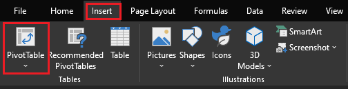
- Highlight cells to create your pivot table.
This time highlight the data or range of cells to summarize in Pivot table. To do this click Insert tab and find the PivotTable command.

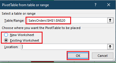
Afterward, the pivottable dialog box will appear which contains the option where you can choose a table or range and where to place the pivot table either in the current worksheet or on another worksheet.
Once you choose a new worksheet you can view it at the bottom of your worksheet. Then Click OK.
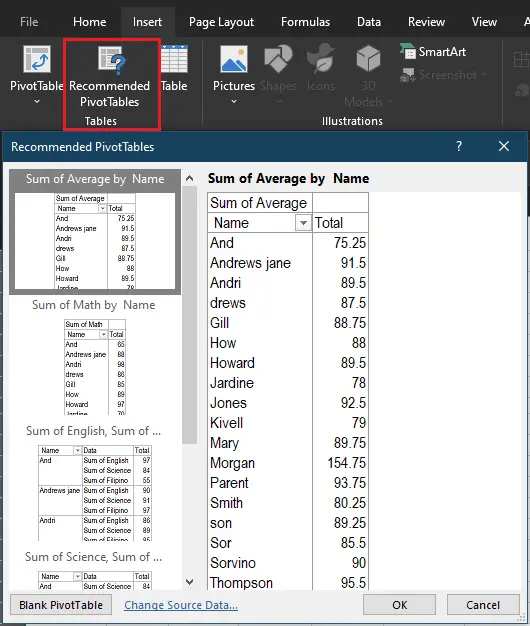
Alternatively, you can highlight your cells, select Recommended PivotTables to the right of the PivotTable icon, and open a pivot table with pre-set suggestions for how to organize each row and column.
- Drag and drop values in the “Row Labels” area.
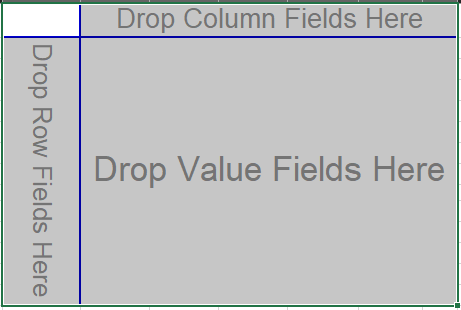
After completing step 3 this will create the blank pivot table.

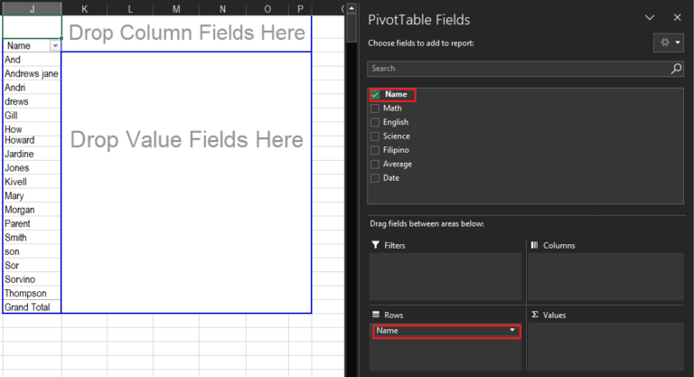
The next thing to do is drag and drop the field which is labeled with the names of the columns in the spreadsheet in the row labels area. This will know what unique identifier the pivot table will organize your data by.
For example, let’s say you want to organize the grades of the student by each subject. To do that, you’d simply click and drag the “Names” field to the “Row Labels” area.
Note: Your pivot table may look different depending on which version of Excel you’re working with. However, the general principles remain the same. - Drag and drop values in the “Values” area.
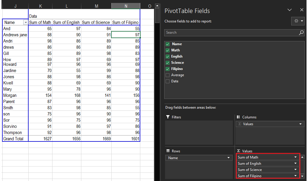
Typically after organizing the data, the next step to do is adding values by dragging a filed values on the Values Area.
With the same example, let’s say you want to summarize average views by grades. To do this, you’d simply drag the subject grades field added to the Values area.
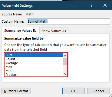
- Change functions for calculations.
Particularly the sum of a certain value will be calculated by default, but you can easily change this to something like average, maximum, or minimum depending on what you want to calculate.

If you are using MAC just click on the small i next to a value in the “Values” area, select the option you want, and click “OK.” Once you’ve made your selection, your pivot table will be updated accordingly.
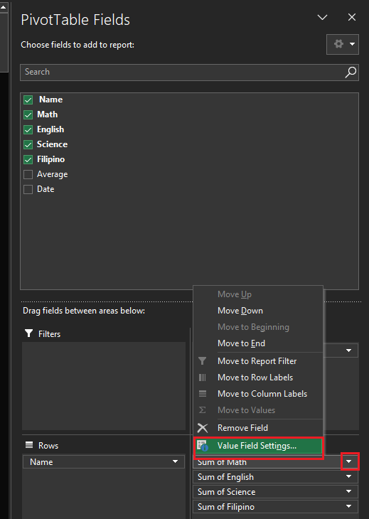
If you’re using a PC, you’ll need to click on the small upside-down triangle next to your value and select Value Field Settings to access the menu.
Conclusion
In conclusion, the article about how to create pivot table in Microsoft Excel is not that complicated, meanwhile it’s great help in summarizing a bunch of data that can not be handled by sorting individually.
Thank you for reading!