What is a Pivot Table?
As mentioned above, a pivot table is an essential Excel feature that helps users organize and summarize complex data quickly.
This feature allows users to group their data by columns, sort it by values, and calculate statistics. In addition, pivot tables are handy when you have a large quantity of data.
How to Create a Pivot Table
If you want to create a pivot table, you should have your data set. Once you have your data, you can start creating pivot tables. Here’s a tutorial on how to make one:
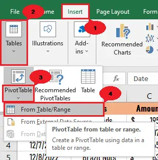
→ Click anywhere on your data, then the Insert tab.
In the Tables group, click PivotTable, then select “from table/range.”
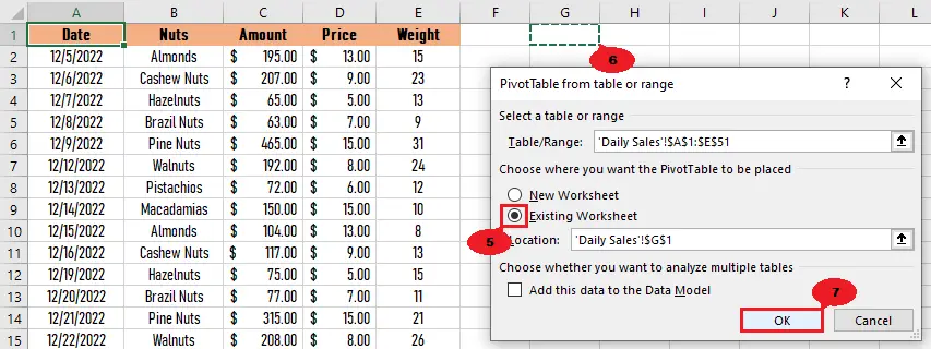
→ After clicking “from table or range,” a PivotTable from table or range dialog box will appear.
Select “new worksheet” if you want to place your pivot table on a new worksheet. However, select “existing worksheet” if you want to place your pivot table on the same worksheet as your data, then select a cell where you want to place it and click OK.
Now that we already understand the pivot table and have even learned how to create one, let’s finally move on to the tutorial.
How to Create a Chart from a Pivot Table
The following is a step-by-step guide on how to create a chart from a pivot table.
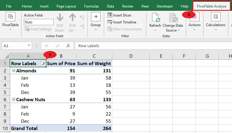
- Click anywhere on your pivot table.
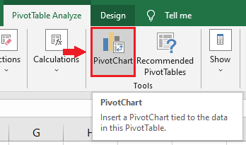
- Click the PivotTable Analyze tab.
After clicking anywhere on your pivot table, click the PivotTable Analyze tab under the PivotTable Tools.
- Select PivotChart.
After doing step two, select the PivotChart in the Tools group.
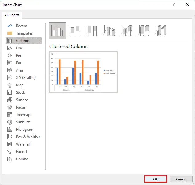
- Edit Insert Chart dialog box.
Lastly, click the OK button in the Insert Chart dialog box.
Note: You can also choose different charts, depending on your preferred chart.
- Result.

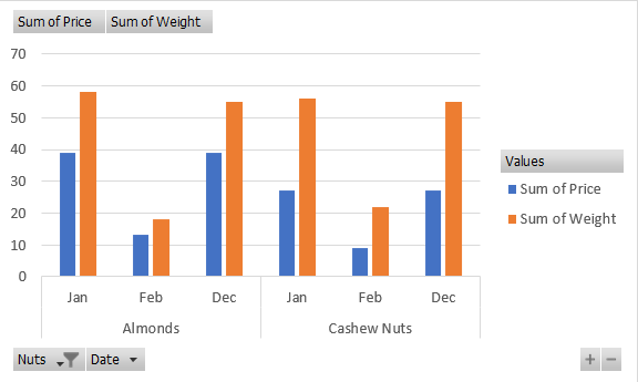
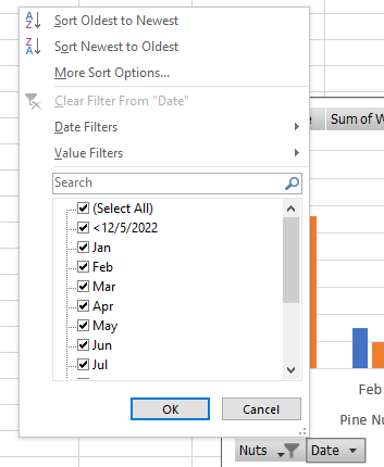
Note: You can filter and choose what to display in your chart by clicking the dropdown button for nuts and date (see image below).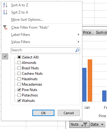
On the other note, you’ll notice a plus and paint sign beside the chart when you click it. They are called chart elements and chart styles. What are these?
- Chart elements. In the chart elements, we can control what we desire to display in our chart.
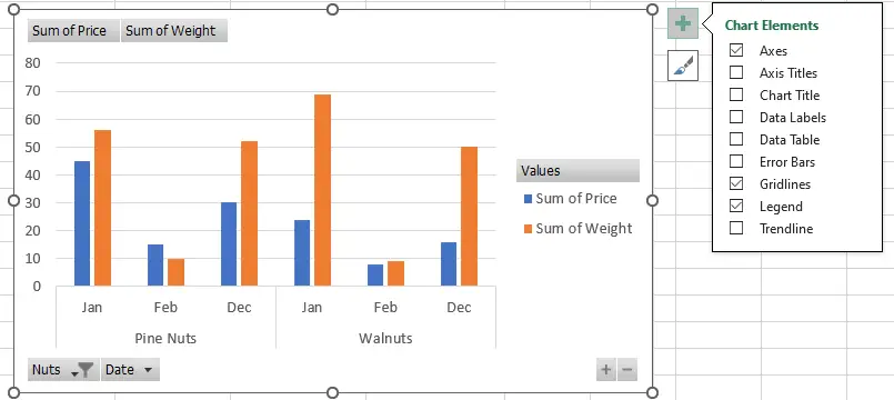
As shown in the picture, you can change (add or remove) the chart elements such as the titles, the data labels, the data table, the error bars, the gridlines, and more. It is done by checking or unchecking the checkbox provided.
- Chart Styles. In the chart styles, we can control the chart style and color scheme for our charts by, of course, clicking on the style and color that we want for our chart.
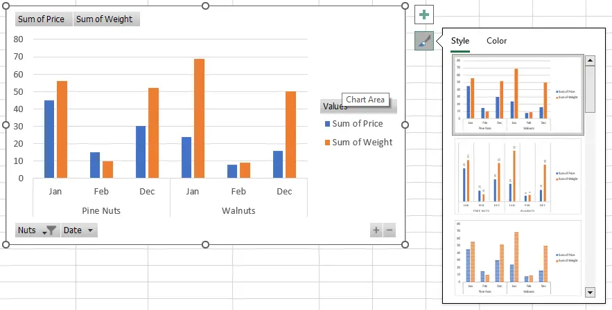
As shown in the picture, you can find different designs or styles by scrolling that scroll panel at the side. And you can also choose a different color for your chart by clicking the color tab.
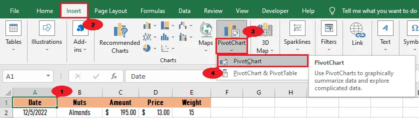
Create a Pivot Chart in Excel
Step 1: Select a cell in your data set, then click the Insert tab.
In the charts group, click the PivotChart button, then select PivotChart.
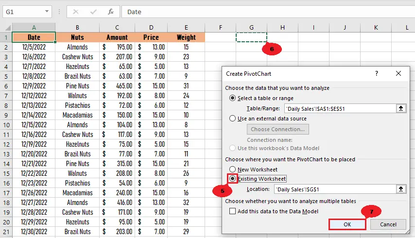
Step 2: After clicking PivotChart, a Create PivotTable dialog box will appear.
Select “new worksheet” if you want to place your pivot chart on a new worksheet. However, select “existing worksheet” if you want to place your pivot chart on the same worksheet as your data, then select a cell where you want to place it and click OK.
Keyboard Shortcut: Click Alt + N + SZ + C keys to show the Create PivotChart dialog box.Conclusion
In conclusion, creating a chart from a pivot table in Excel is easy and quick. Learning how to do it is also an easy thing to do.
By following the simple steps in this article, there’s no doubt that you’ll learn it quickly.
I believe that we have accomplished this tutorial. I hope you’ve learned something from this. Do not forget to share this with your friends.
If you have any questions or suggestions, please leave a comment below.

Elijah Galero
Programmer & Technical Writer at PIES IT Solution
Elijah Galero is a programmer and writer at PIES IT Solution, author of 175+ tutorials at itsourcecode.com. Specializes in Python error debugging (AttributeError, TypeError, ModuleNotFoundError), Python programming tutorials, and Microsoft Excel how-to guides for BSIT students and productivity learners.
Expertise: Python · Python Errors · Python AttributeError · Python TypeError · ModuleNotFoundError · MS Excel · MS PowerPoint · View all posts by Elijah Galero →