In this article we discuss how to multiply columns in excel with help of example data and figures, hence will be easy for you to understand and learn.
So in our last tutorial, we learn how to subtract in Excel. This time we will proceed to multiplication as we go along we will elaborate on all possible ways and features
Based on the prior tutorial we mentioned that Microsoft Excel is designed to manipulate numbers, and can able to calculate different operators of basic math. Additionally, it can handle a handful of information.
What is the Formula for Multiplication in Excel
Excel has no specific formula for multiplication but there’s a way you can do to execute multiplication. Namely the asterisk (*) a mathematical symbol used in multiplication and product function to multiply(=product). Further, there are a lot of ways to multiply cells and numbers you can try in this topic.
How to do a Multiplication Formula in Excel
Using the mathematical symbol (*) is the easiest way to create a formula in excel. With this approach, you can multiply numbers, cells, or entire columns and rows.
Here is how to…
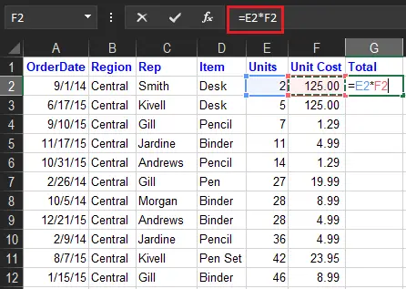
We will multiply two cells in the first row. Assuming we will select cell in your data in row 2 and in columns E And F. So we will put the result in cell G2. Therefore the formula is simple as this =E2*F2.
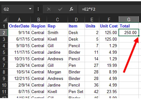
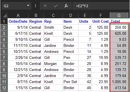
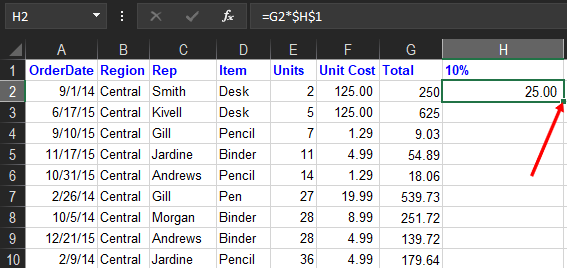
After that to make it faster just double-click the green square to copy the formula in the rest of the cells and you’re done.
This happens because we are using relative cell reference which does not have a ($) sign along with it the references will be changed based on the row where the formula is placed. For instance, the formula in the cell G3 will be =E3*F3.
How to Multiply Two Columns in Excel
There are two easiest ways to multiply two columns in Excel. This is by using mathematical symbols and the PRODUCT functions.
So in this case, if you want to use the mathematical symbol (*) the same step is performed above, however…
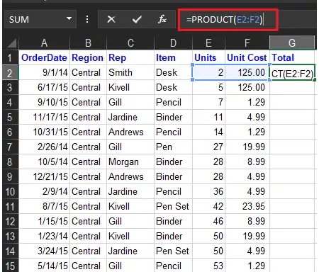
If you prefer working with Excel functions rather than expressions, you can multiply 2 columns by using the PRODUCT function, which is specially designed to do multiplication in Excel.
For our sample data set, the formula goes as follows:
=PRODUCT(E2:F2)
As with the multiply symbol, the key point is using relative cell references, so that the formula can adjust properly for each row.
You enter the formula in the first cell and then copy it down the column as explained in the above example.
How to Multiply Multiple Columns in Excel
To multiply more than two cells or columns in Excel is similar to how you multiply two columns, but this time you will just add more range of cells and columns.
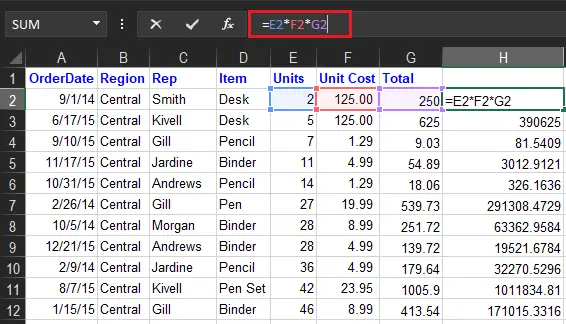
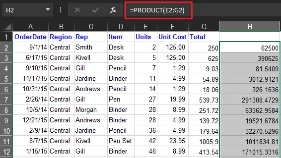
For example, to multiply values in columns E, F, and G, use one of the following formulas:
- Multiplication operator:
=E2*F2*G2
- PRODUCT function: =PRODUCT(E2:G2)
- Array formula Press Ctrl+Shift+Enter: =E2:E15*F2:F15*G2:G15
As shown in the screenshot above, the formulas multiply numbers and decimals very well.
How to Multiply a Column by a Number in Excel
This time we will multiply the same number in all values in a column. As we know the fastest way to do multiplication is using its sign operator (*).
To begin here are the following ways we can use to execute this task.
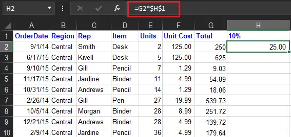
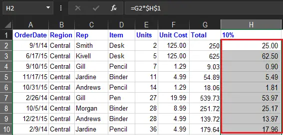
- Enter the number you want some cell to multiply, say in H1.In this case, we are going to multiply a column of numbers by a percentage.
- Write a formula for the topmost cell in the column or formula bar, locking the reference to the column of constant number with the dollar sign ($) (like $H$1). Therefore, the formula goes as follows:
=G2*$H$1. - Input the multiplication formula in the topmost cell (H2) and press Enter Key on your keyboard.

- Double-click the small green square in the lower-right corner of the formula cell to copy the formula down the column as far as there is any data to the left. That’s it!
An absolute cell reference is when the dollar sign is in between the cell reference($H$1), thus it’s utilized to fix the row and column coordinates of number you want to multiply. Hence, the reference does not change when copying the formula to the other cells.
As a result, the formula in H2 changes to=G2*$H$1, the formula in H3 changes to =G3*$H$1, and so on.
Summary
In summary, we covered how to multiply columns in Excel as well as its formula. Other than that there are a lot of ways you can perform multiplication in Excel using its operator and product function that is convenient for doing our task.
Thank you for reading!


