In this tutorial, we will know what is Excel relative cell reference and how to use it. Along with how it differs in absolute reference in excel.
Usually, we use a cell reference to locate the cell address or name of a cell or range of cells. Apparently, these are the combination of column names and number of rows. This helps excel to determine from what and where data or value to be used in the formula.
What is Relative Reference in Excel
A relative reference in Excel is a default cell you can see in every formula. Specifically, this cell reference is the one without the $ sign, like G2.
So when using relative cell reference copied to another cell definitely the cell reference changes based on the relative position of rows and columns.
Particularly, all references are relative. Let me show you how relative reference works:
Assuming we select cell B2 to put our formula:
=A2*B2
Therefore if you copy this formula to another cell, this will adjust to another row like A2 will be A3 and B2 will be B3 which Excel assumes you want to multiply the succeeding cells.
Relative Reference Example
After we define what is a relative reference we are going to do now examples. So that we can understand how it works.
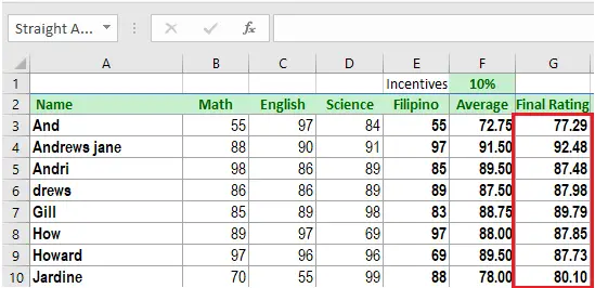
Assumingly, we have 10% incentives and a list of average that needs incentive points to obtain a final grade.
So to create formula we have the reference of the average and the 10% incentives.
Take a look at the given formula:
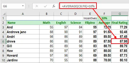
=AVERAGE(C3:F3)+10%
Notice, that we are using an Excel relative cell reference, without the dollar sign.
How to use Relative Reference in Excel
In the following example, we want to create a formula that will multiply the average by the given 10 % incentives. Instead of creating a new formula for each row, we can just copy the formula to the next cell. We’ll use relative references so the formula correctly calculates the total for each item.
Time needed: 2 minutes
So here are the step by step on how to use relative reference in Excel.
- Select a cell where you want to input the cell.
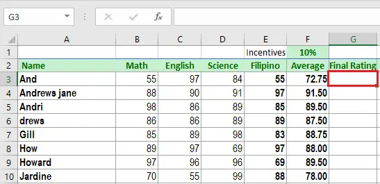
Click an empty cell that will contain the formula. In our case, we select cell G3.

- Type the formula you want.
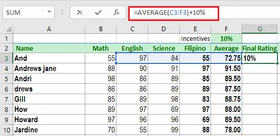
Enter the formula to calculate the desired value. In our example, we enter =AVERAGE(C3:F3)+10%.

- Press Enter on your keyboard
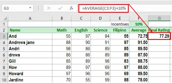
On your keyboard Press Enter key. This will display the result of the formula entered in the specified cell. Then, locate the fill handle in the lower-right corner of the selected cell. In our example, we’ll locate the fill handle at cell G3.

- Use the fill handle to copy formula.
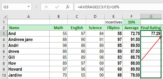
To copy the formula on the succeeding cell, click, hold and drag the fill handle over the cells you want to fill. For instance, we drag fill handle from G3:G10.

- Release the mouse from hold.
Upon releasing the mouse, the formula will be copied to the selected cells with relative references and the values will be calculated in each cell.

- Check the accuracy of the formula.
To check the accuracy of the relative reference in the formula. Just double-click the cell containing the result. Suppose each relative should be different on each cell depending on its row.

Difference between Absolute and Relative Reference in Excel
The difference between the absolute, relative and mixed cell reference is explained below.
- The relative reference is the default location of a cell. Wherein the row and column are not fixed that when you drag or copy the formula it changes subsequently. Meanwhile…
- An absolute reference is a fixed or absolute location of the cell like $A$1, $B$2, and so on. The row and column both are kept constant in an absolute reference. Thus,
- A mixed reference is one in which either the row or the column is kept constant like A$2, $D2, and so on.
Conclusion
We hope this article has clarified how to use a Relative reference in Excel. This topic may be difficult to grasp at first, but it is critical if you want to improve your Excel skills.
Thank you for reading 🙂


