In this tutorial we are going to explain what is AND function of Excel and How to use it basically and with other functions. Along with are examples that will cover AND function and images that show how it works.
What is AND function in Excel?
The Excel AND function is a logical function which is used to have and test multiple conditions at the same time. This returns TRUE or FALSE. Moreover, this function can take up 255 conditions and check more than one logical condition at the same time.
Further, each argument expression of AND function must be evaluated as TRUE or FALSE. In every expression, it could be a cell reference, constant, arrays or logical expression.
Syntax
=AND(logical1, [logical2], …)
Arguments
logical1 – The first logical value or condition to evaluate, it is required.
logical2 – This is the second condition, it is optional.
Return value
Returns TRUE if all the arguments are evaluated as TRUE otherwise FALSE.
The Logic of AND function
| Formula | Return Value |
| =AND(TRUE,TRUE) | TRUE |
| =AND(TRUE, FALSE) | FALSE |
| =AND(FALSE, FALSE) | FALSE |
| =AND(FALSE, TRUE) | FALSE |
Excel AND function Characteristics
- If all the arguments in functions are all TRUE then logical functions will be evaluated as TRUE.
- If any of the logical function’s arguments or values is FALSE, then it will return FALSE.
- It can contain more than one logical value depending on the requirements or certain conditions.
- If the value is zero it will read as False and all non-zero values are evaluated as True in evaluating numbers.
- It is mostly used with other Excel functions such as IF, OR and more.
Excel And Function Limitations
The following lists are limitations of AND function:
- Excel version 2007 and higher can handle up to 255 arguments as long as the characters of the formula do not exceed 8,162 characters.
- On the other hand, the previous version of Excel 2003 can only hold 30 arguments wherein the argument characters can on take up to 1,024 characters.
- Returns #VALUE! error if the arguments are not evaluated in a logical value, or the logical conditions are handed as text.
- If the values of the arguments are on empty cells Excel AND function will return #VALUE! error.
How to do And Function in Excel
Working with AND function can be easy as possibly. And now let’s understand how this function works with these few examples.
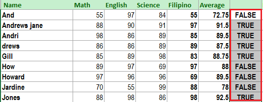
Assuming we have the given data which contains the grades of students. So what we have to do is to determine if their grades in each subject are greater than or equal to 80.
The given data is as follows:
So we will apply the formula to the cell or column we prefer, in our case we enter the formula in column G.
Then the result of the formula will appear in column G.
As we can see there are four students who do not reach 80 grades in their subject. Wherein the first student only got 55 grades in his Math and Filipino subject. The reason why the return is False.
The same manner happens to the three students which How got only 69 in his Science subject while Howard got 69 on his Filipin and Jardine Math subject grade only 70. Therefore if all of these subjects reach 80 and above grades this will return True.
IF AND function in Excel
Now let’s consider this scenario on how the IF and AND functions of Excel work.
Prior here is the syntax of IF function:
=IF(logical_test,[value_if_true],[value_if_false])
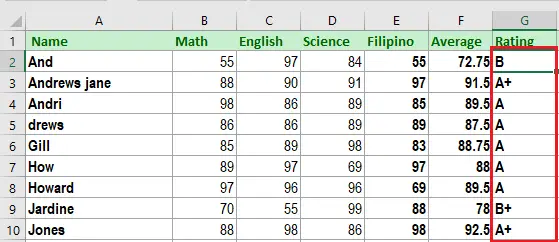
So we have here the Final grades of students, where we need to determine the grade of students according to the criteria given.
And now the student who gets an “A+” must acquire more than 90%. Hence if the percentage is greater than or equal to 80% but less than or equal to 90%, the criteria for the grade given is “A”.
Further, if the grade is less than 40% is failed. Likewise, the grades for the different percentages are given in the following table.
The formula we are going to apply is given below:
=IF(F2>90,"A+",IF(AND(F2<=90,F2>80),"A",IF(AND(F2<=80,F2>75),"B+",IF(AND(F2<=75,F2>70),"B",IF(AND(F2<=70,F2>60),"C+",IF(AND(F2<=60,F2>50),"C",IF(AND(F2<=50,F2>40),"D","FAIL")))))))
Particularly, the IF function will return TRUE if the condition is met otherwise it will return false.
The first logical value is “F2>90.” If this condition is TRUE, the grade “A+” is indicated. If this condition is FALSE, the IF function evaluates the next condition.
The next logical test is “F2<=90, F2>80.” If this condition is “true,” grade “A” is assigned. If this condition is “false,” the next statement is evaluated. Likewise, the IF function tests every condition given in the formula.
The last logical test is “F2<=50, F2>40.” If this condition is “true,” grade “D” is assigned, else the student fails.
The output of the formula is given below:
Conclusion
In conclusion here is the following summary about And Function of Excel.
- This function is not case-sensitive. Thus…
- And Function ignores values or empty cells argument.
- Returns #VALUE if the logical values are not found during the evaluation.
Thank you for reading 🙂


