
In this tutorial, we will explore more about the sum function of excel which we provide examples and explanations on how it works.
What is the sum function in Excel?
The sum function formula of excel is used to add the numerical values in a range of cells. The value that can be supplied in functions either in cells, references, or range of cells. So this function is used in a situation when it is required to total selected cells.
In addition, this function SUM can handle up to 255 individual arguments.
The Syntax of the SUM Excel Function
The syntax of the sum is shown below:
=SUM(number1, [number2], [number], …)
Arguments
This function accepts the arguments as follows:
- number1 – The first value to sum.
- number2 – [optional] The second value to sum.
- number3 – [optional] The third value to sum.
How to Use Sum Function in Excel
Time needed: 5 minutes
Primarily, to use the sum function you just need to type (=SUM) followed by the arguments. However, we provide you here the alternative steps on how to use the sum function of excel.
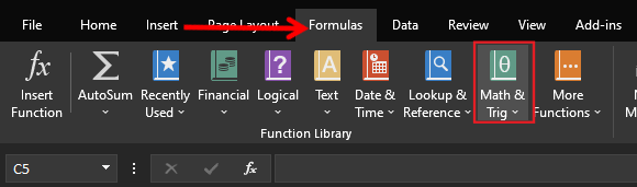
- In the Formulas tab, click the “math & trig” option, as shown in the following image.
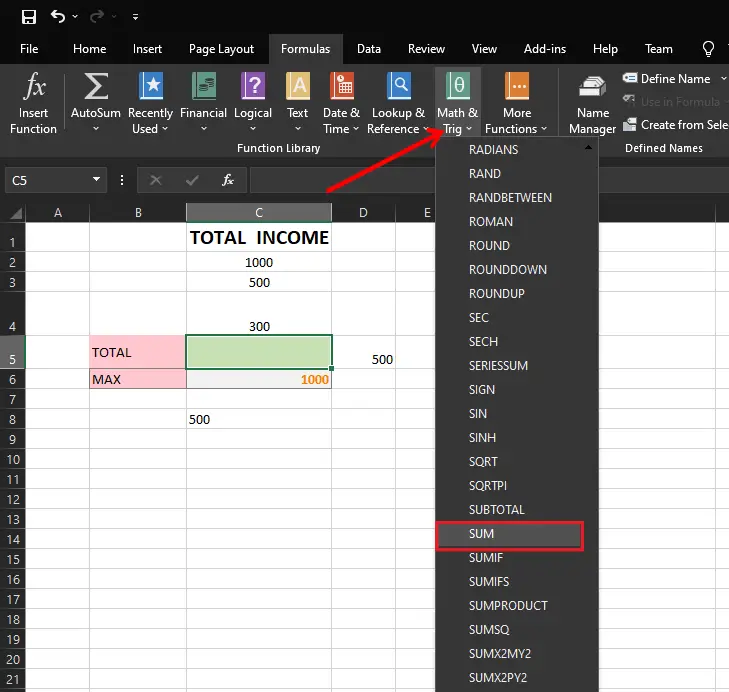
- From the drop-down menu that opens, select the SUM option.
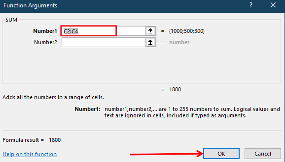
- In the “function arguments” dialog box, enter the arguments of the SUM function. Click “Ok” to get the output.
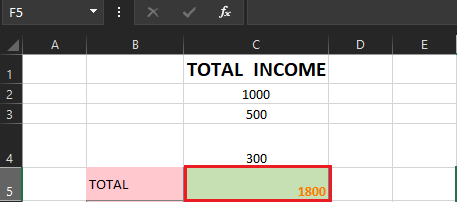
- Here’s the output.
Excel SUM Formula Examples
Here we will give a few examples to understand how to use it in different ways, thus we will provide figures to answer clarification.
Example 1
In this example, we will use Autosum button which is the quickest and easiest way to sum up a range of cells. Once it is used Excel sum function automatically enters on selected cells. As defined above it totals one or more numbers in a range of cells.
The first example, below, shows how to use the AutoSum feature.
| Steps | Figures |
| 1. First, select a blank cell you want sum below the cells of the row. | 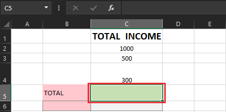 |
| 2. On the Home Tab Click the Autosum button or Alt+= on your keyboard. | 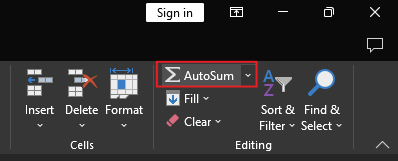 |
| 3. Then in your active cell A SUM formula will appear, with a reference to the cells above. In our figure, the formula in C5 is (=SUM(C2:C4). Note: You can extend the frame if your cells are not included. | 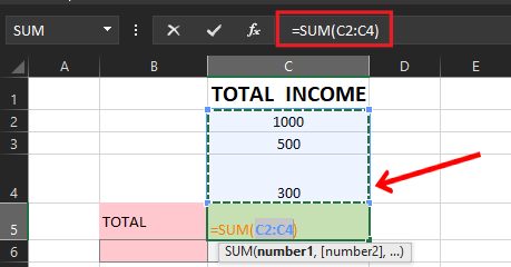 |
| 4. Click Enter Key then the result will display. | |
Example 2
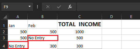
Normally, the SUM function is often used in bigger and more complex calculations. So let’s assume here the given data.
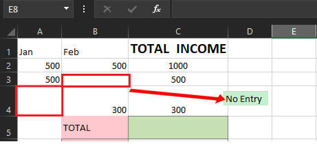
The illustration above shows a piece of missing information in a worksheet; now let’s use the sum function with IF function to display a warning message.
Here is the formula we used.

We get the result below:
Excel SUMIF Formula
The SUMIF function of excel calculates the sum value of the range of cells with true or false conditions.
The syntax of this function is SUMIF(range, criteria, [sum_range]).
SUMIF Two Required Arguments
- range – cells to check for the criteria
- criteria – value to use as criteria
SUMIF Optional Arguments
- [sum_range] – cells to sum if omitted, values in range are summed
- These arguments can be cell references or can be typed into the formula.
Example Excel SUMIF Formula
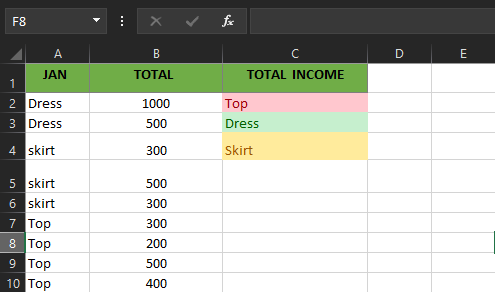
In this example, we will know how to calculate using SUMIF and meet a specific criterion or multiple criteria. Consider the following given data in Excel table to calculate each income.
- Select the cell in which you want to see the total
- Input an equal sign (=) to start the formula
- Type: SUMIF(
- Select the cells that contain the values to check for the criterion.
- Type a comma, to separate the arguments
- Select or type the criterion.
- Type a comma, to separate the arguments
- Select the cells that contain the values to sum.
- The completed formula is:
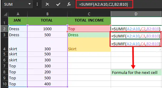
=SUMIF(A2:A10,C2,B2:B10)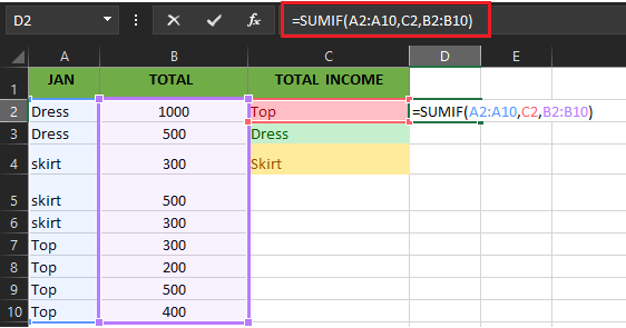
- Press the Enter key to complete the entry
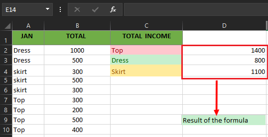
Note: Instead of typing the criterion in a formula, you can refer to a cell. For example, the formula in step 9 above could be changed to: =SUMIF(A2:A10, C3, B2:B10)
Excel Sum Formula Shortcut
Suppose we have values in more than one column, so how can we add this numerical value?
Here’s how…
- First, you must select all the columns you want to add.
- Then, Press “Alt+=”.
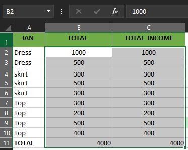
Now it has already applied the formula to the last cell selected. Note do not press the ENTER KEY instead pressing CTRL+ENTER to apply the formula on the same selected cell.
Hence the result is presented below after using the shortcut keys.
Horizontal Auto Sum in Excel
This time we also have a horizontal Autosum shortcut way. As we’ve seen how to apply it is a vertical set of data it is more likely the same as how it is done.
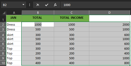
- First, Select the cell you want to be total, for instance B2 to C10.
- Then Press the excel Sum shortcut, Alt+=.
As we can see, it has applied the Excel SUM formula shortcut to the beside cell of the selected cells.
Summary
In summary SumFunction of Microsoft excel helps the summation easier; it also considers adding a numerical set of data with a condition considering the possibility when doing tasks or financial reports specifically.
Thank you for reading!