
In this tutorial, we will elaborate what is SUMIFS function can do in Excel worksheets. Along with different examples, formulas and different criteria where SUMIFS function can be used.
What is the SUMIFS function in Excel
The Excel SUMIFS function sums cells range that meets more than one condition or criteria. This function supports logical operators and wildcards. Additionally, this function is a widely used function. The good thing about this it can sum up cells based on dates, number values, and even text.
Syntax
=SUMIFS(sum_range, criteria_range1, criteria1, [criteria_range2, criteria2] ...)
Technically, the syntax of this function clearly depends on the required conditions. Thus every separate condition requires range and criteria.
Arguments
- sum_range – It is the range of cells to be summed.
- range1 – It is the first range to evaluate.
- criteria1 – It is the first range criteria.
- range2 – An optional, it is the second range to evaluate.
- criteria2 – Optional, it is the criteria on the second range.
To clearly understand these arguments, the sum_range which is the first one it must contain numeric value wherein it is the range to sum up. While the second argument is the range1 where the first condition happens.
Then the third argument is the criteria1 of the first condition of the arguments, together with logical operators. Subsequently, the same logic to the next range and criteria.
Return Value
The sum of cells that meet all criteria.
Apparently, SUMIF and SUMIFS function supports wildcards and logical operators, in partial matching. Thus this function syntax is a little bit tricky because SUMIFS functions split logical criteria into two parts.
Hence, each condition requires a separate range and criteria. Thus, operators need to be enclosed in double quotes (“”).
The table below shows some common examples:
| Target | Criteria |
|---|---|
| Cells less than 75 | “<75” |
| Cells equal to 95 | 95 or “95” |
| Cells greater than or equal to 95 | “>=95” |
| Cells equal to “Branch A” | “Branch A” |
| Cells not equal to “Branch A” | “<>Branch A” |
| Blank Cells “” | “” |
| Cells that are not blank | “<>” |
| Cells that begin with “A” | “A*” |
| Less than B2 cells | “<“&B2 |
| Greater than today cells | “>”&TODAY() |
Basic SUMIFS Excel Formula
Now we will create a basic SUMIFS formula, we will use this to sum G3:G11 and equal to Branch A.
=SUMIFS(G3:G11,A3:A11,"Branch A")
If the range B3:B11 contains Product names like “Product 1”, “Product 2”, and “Product 3”, you can use SUMIF to sum numbers in G3:G11 when the product name in B3:B11 is “Product 1” like this:
=SUMIFS(G3:G11,A2:A11,"Branch A", B3:B11, "Product 1")
The arguments we have now are five, sum_range is G3:G11, range1 is A3:A11 and criteria1 is “Branch A”, and range2 is B3:B11 and criteria2 is “Product 1”.
So here is the illustration in the worksheet example.
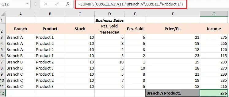
As you notice putting equal to sign (=) is not necessary for constructing formula criteria. Thus it is not case-sensitive, you can type either— branch a or Branch A.
Visit also Excel Sum Function to know more basic and AutoSum function.
SUMIFS Excel Example
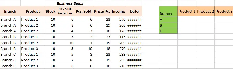
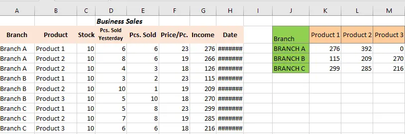
Suppose we want to calculate the total income for each product across three different branches. Here, our first criterion is the Branch and the second criterion is the product.
The following are the steps to calculate the total income along with SUMIFS function.
- The given data includes Branches and Products and removes duplicate values. Thus it should look likes below.
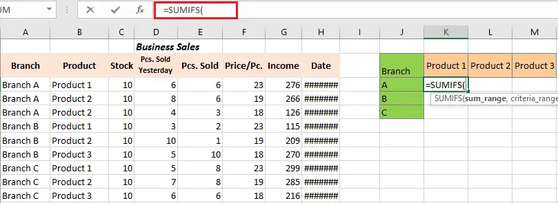
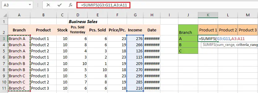
- Now utilize SUMIFS function in the worksheet. Enter SUMIFS function in Excel.
- Highlights the sum_range as G3 to G11.
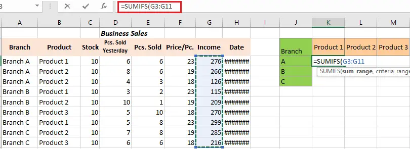
- Highlights the A3 to A11as the “criteria_range1.”
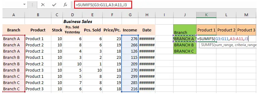
- The range 1 “criteria” will be the “Branch A.” Then, choose cell H2 and lock only the column.
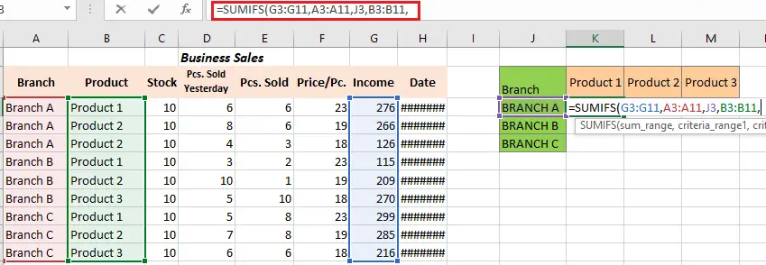
- Then highlight the “criteria_range2” that will be B3 to B11.
- Hence the “criteria_range,” is “Product 1,” so select the K2 cell as the reference and lock the only row here.
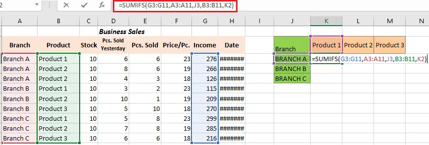
- And now we have value for the Branch “Branch A” and the Product “Product 1″ and the rest.
SUMIFS date range
Whenever to sum cells within the dynamic range of date, create criteria by using TODAY function. This will get the current date and automatically updates it.
For instance, to sum income within the last 7 days including today’s date, below is the formula:
=SUMIFS(G3:G11,H3:H11, "<="&TODAY(), H3:H11, ">"&TODAY()-7)
Hence if you don’t want to include the current in the final result. Utilize less than operator on the first criteria in order to exclude today’s date. Thus on the second criterion use greater than or equal to include the date which is before 5 days of the current date.
=SUMIFS(G3:G11, H3:H11, "<"&TODAY(), H3:H11, ">="&TODAY()-5)
Meanwhile, to sum cells value with dates on given days forward.
Take a look at this example, we will get the total income in the next 2 days, the formula is as follows:
=SUMIFS(G3:G11,H3:H11, ">="&TODAY(), H3:H11, "<"&TODAY()+2)
Here on the result, today’s date is included. The next formula is today’s date is not included.
=SUMIFS(G3:G11, H3:H11, ">"&TODAY(),H3:H11, "<="&TODAY()+2)
SUMIFS between Two Dates
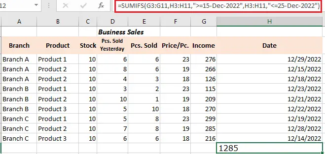
Here you have sales data for the month of December, and you need to sum values between 15-Dec-2022 to 25-Dec-2022.
In your preferred cell input the following formula, in our case cell H12.
=SUMIFS(G3:G11,H3:H11,">=15-Dec-2022",H3:H11,"<=25-Dec-2022")
As you press enter key, you get 1285 result in the cell which is the sum of the amount between 15-Dec-2022to 25-Dec-2022. Wherein the calculation indicates both start and end dates as well.
Conclusion
In conclusion Excel Sumifs function is a powerful tool which can be very efficient when worksheets need to sum data having multiple criteria or conditions to meet. Since you know how useful it is, you cannot avoid this now to use in certain situations.
Thank you for reading 🙂