
In this tutorial, we will learn how to add sparklines in Excel in a short period of time. Aside from that, we will also learn about its types and how to customize them.
When working with Excel, it is crucial to know its functions and what it can do. It is for us to make our job easier and more efficient. That is why we are here to help you on your Excel learning journey.
On a different note, let’s first briefly understand sparklines.
What are Sparklines in Excel?
A sparkline in Excel is a small chart placed in a single cell. This represents a row of data in your selection. We use this chart to display trends.
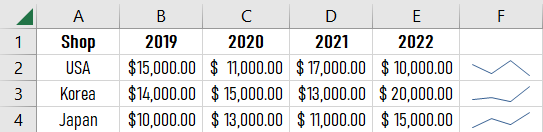
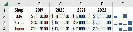
This chart is not an object and isn’t the same as the regular charts. Here’s an example of data with sparklines:
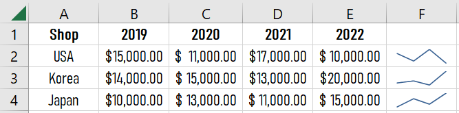
In the sample above, we can see the difference in the revenues of a shop every year and in its branches in other countries.
Note: The sample above is just an example and isn’t based on actual research or business.
Anyway, let’s not prolong the discussion any longer and jump right into our tutorial.
How to add Sparklines in Excel (Tutorial)
Time needed: 1 minute
Here’s a step-by-step guide on how to add sparklines in Excel.
- Open Excel and input the data.
The first thing we should do is open a blank Excel worksheet, then input your data.
Note: If you already have your data in an Excel sheet, skip this step.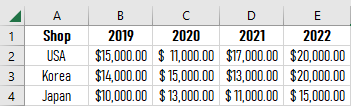
- Select the cells where you want your sparklines to display.
The next step after entering our data is to choose the cells where we wish to display our sparklines.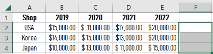
- Click the Insert tab, then the Sparklines button.
Once cells are selected, click the insert tab above and then the sparklines button. Then you’ll see the three types of sparklines: line, column, and win/loss. Select the line option.
Note: You can select any of the three (line, column, or win/loss), but we’ll use line sparklines in this tutorial.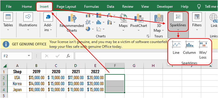
- Select the data range, then click OK.
A dialog box will appear after clicking the line button, and that’s when we select our data range. Then click OK.
Note: You can manually input the data range by typing it in the textbox next to the “data range” label.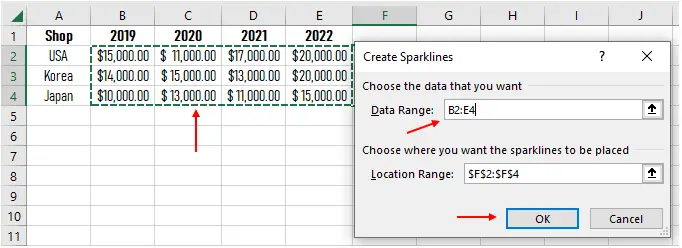
- Result.
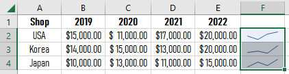
Tip: Excel automatically updates the sparkline if you change your data.Customizing Sparklines
In this part, we will learn how to customize our sparklines. We’ll learn how to put markers in it, how to highlight its high and low points, change its color, etc.
Here’s how we customize our sparklines:
STEP 1: Select the sparklines.
STEP 2: Click the Sparkline tab. After clicking the Sparkline tab, here’s what you’ll see:
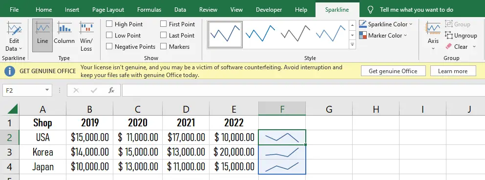
There, we can edit its location and data, change its type, show points and markers, change its style and color, edit its axis, group or ungroup it, and clear the selected sparkline.
Types of Sparklines
Sparklines are classified into three (3) types. These are the line sparkline, column sparkline, and win/loss sparkline.
1. Line Sparkline
2. Column Sparkline
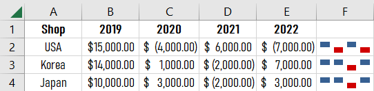
3. Win/Lose Sparkline
Conclusion
In conclusion, this tutorial is a key to making our work in creating or adding a sparkline in Excel easier and more effective.
I think that’s it for this tutorial. I hope you’ve learned something from this. If you have any questions, please leave a comment below, and for more educational content, visit our website.
Thank you for reading!