
In this tutorial, we will learn how to create bar chart in Excel, along with creating different bar chart types and customizing chart appearance.
Likewise other charts such as pies, bar, and line charts, or commonly used charts. These are easy and simple to understand. After this tutorial, you will know what best bar charts are suited to your worksheets. Further it is working in any numerical data you want to compare such as percentage temperatures, frequencies or other measurements.
What is Bar chart in Excel?
A bar chart (bar graph) in excel is used to visualize distinct categories of data in rectangular bars. The lengths of these bars are proportionate to the presented size of the data category.
Further, this graph can be plotted in vertical or horizontal style, and the vertical bars are separate type of chart which is called column bar charts.
How to make a bar chart in Excel
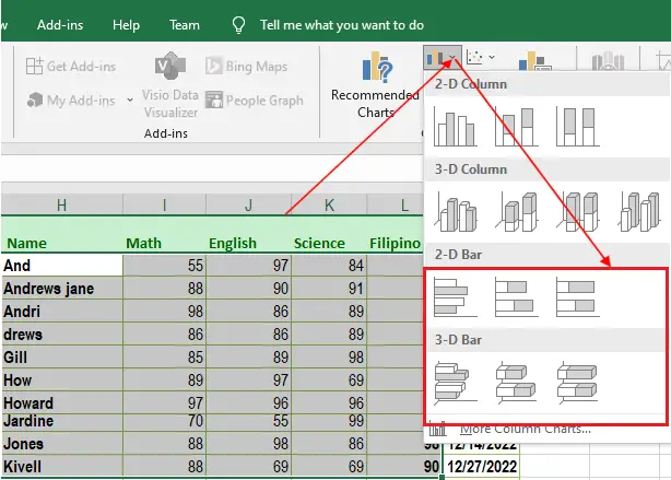
Making a Bar chart in Excel is easy as possible. The only thing you have to do is ready your data wherein you gonna plot the chart. Go to Insert tab>Chart group in the ribbon tab and select the bar chart you want.
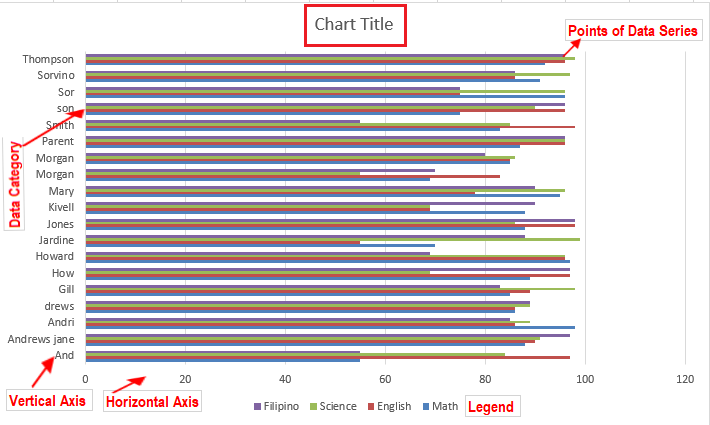
Here is an example of Bar Chart:
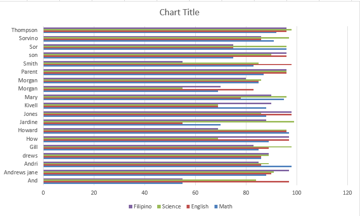
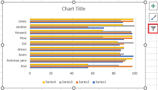
The chart above displays multiple data series wherein the source of data we have contains two or more columns of numerical values, hence each shaded in a different color.
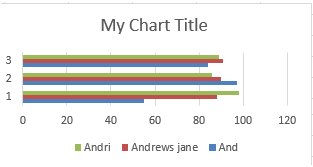
Meanwhile, if you want to display only one data series your source of data must only have one column of numbers. Thus, we will select the default 2-D clustered chart bar.
Formatting Bar Charts in Excel
After creating the bar charts, apparently there is a lot of formatting you can change such as the color, the style, changing the title of the chart or even editing axis or adding an axis label on each side.
Change Bar Graph Title
In changing the bar chart or graph title you have to double click the text box on the upper portion of the chart. Then you can be able to edit or change your chart title.
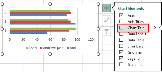
Then if you want to completely remove the chart title, click anywhere in the chart and when you see the Plus sign icon, it’s the chart element. Then uncheck the checkbox next to the Chart title.
Changing Bar Chart Style and Colors
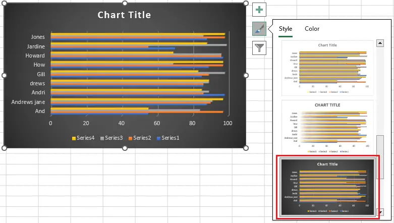
Aside from changing title of the chart, Microsoft Excel also provides different themes which you can utilize in your bar chart. To use this click anywhere in your chart and click the chart style in a paintbrush icon.
Further, the list of themes will appear. Select the style to modify the appearance of your chart including the layout and background.
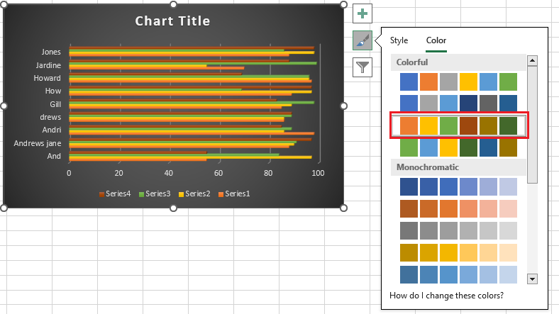
In our case, we select style number 9 which has a black radiant background, see the figure below.
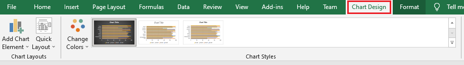
In addition to this, we can also have these styles on the Design Tab under the chart tools section in the ribbon bar. In the same manner, you can see the preview of the chart when you select the chart style available in the ribbon.
Obviously changing of color of the chart is provided also under the section of Chart style menu “Color”. As you optimized take note that these colors are grouped, so you will select the color palette to apply on charts.
Color options are grouped, so select one of the color palette groupings to apply those colors to your chart. The good thing is you can see the preview of the color palette as you hover the mouse.
How to create different bar chart types in Excel
Whenever you are making bar charts, you can choose the chart types you prefer. So, here are the possible charts you can utilize.
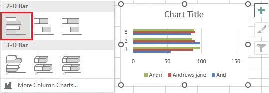
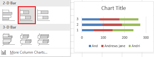
Clustered bar charts
The clustered bar charts of excel feature comparable values across data categories. Typically the categories of the data are organized together with their vertical axis (Y-axis) and along with the horizontal axis (x-axis).
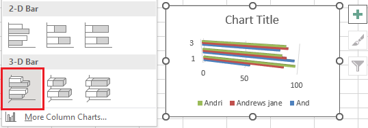
Meanwhile, the 3-d clustered bar charts do not include the third axis but present the 3-D format of horizontal rectangles.
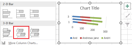
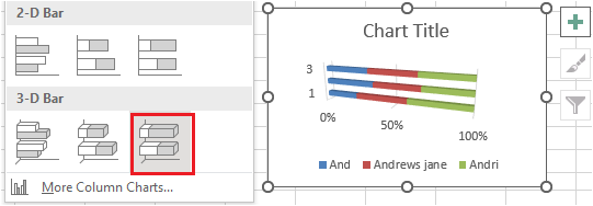
Stacked bar charts
A stacked bar graph in Excel shows the proportion of individual items to the whole. As well as clustered bar graphs, a stacked bar chart can be drawn in 2-D and 3-D format:
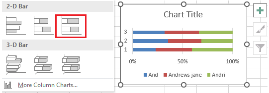
100% stacked bar charts
This type of bar graph is similar to the above type, but it displays the percentage that each value contributes to a total in each data category.
Conclusion
Wrapping up this article covered the Bar chart of excel which typically a helpful one in visualizing data. Asides, this chart is good in comparing and distinguishing the distinct of data values in rectangular bars.
There you have it! We finish the guide how to add bar charts in Excel. If you have any clarification about this or any other Excel feature, let us know in the comments. We are always happy to help.
Thank you 🙂